Pattern Classification All materials in these slides were

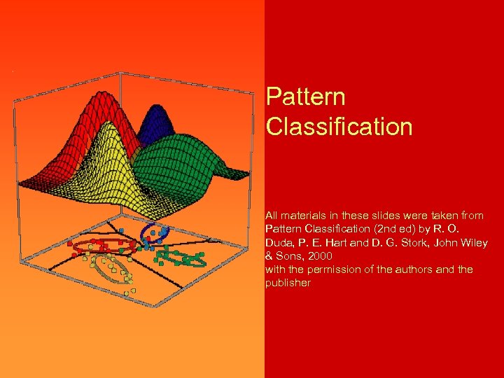Pattern Classification All materials in these slides were taken from Pattern Classification (2 nd ed) by R. O. Duda, P. E. Hart and D. G. Stork, John Wiley & Sons, 2000 with the permission of the authors and the publisher

Bayes decision theory febr. 17.

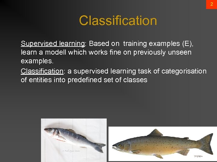2 Classification Supervised learning: Based on training examples (E), learn a modell which works fine on previously unseen examples. Classification: a supervised learning task of categorisation of entities into predefined set of classes

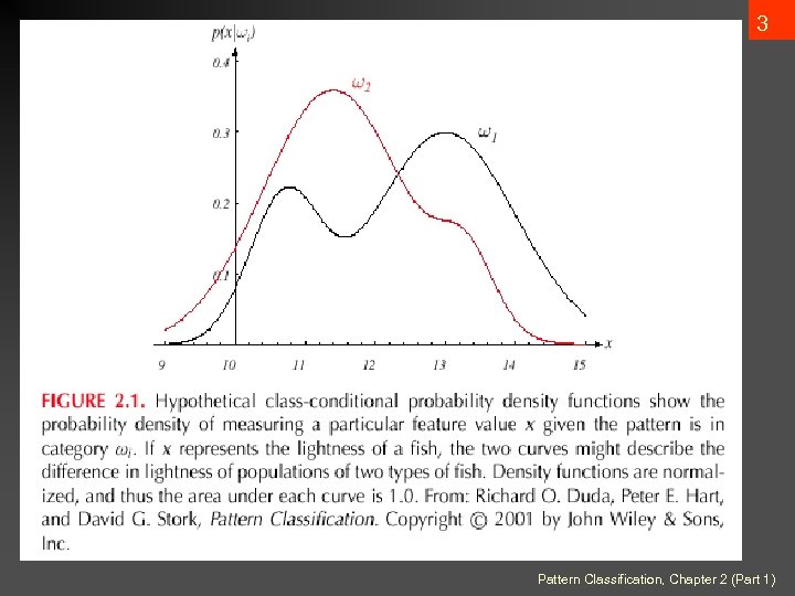3 Pattern Classification, Chapter 2 (Part 1)

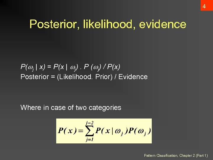4 Posterior, likelihood, evidence P( j | x) = P(x | j). P ( j) / P(x) Posterior = (Likelihood. Prior) / Evidence Where in case of two categories Pattern Classification, Chapter 2 (Part 1)

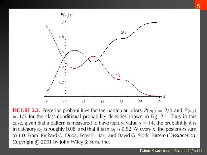5 Pattern Classification, Chapter 2 (Part 1)

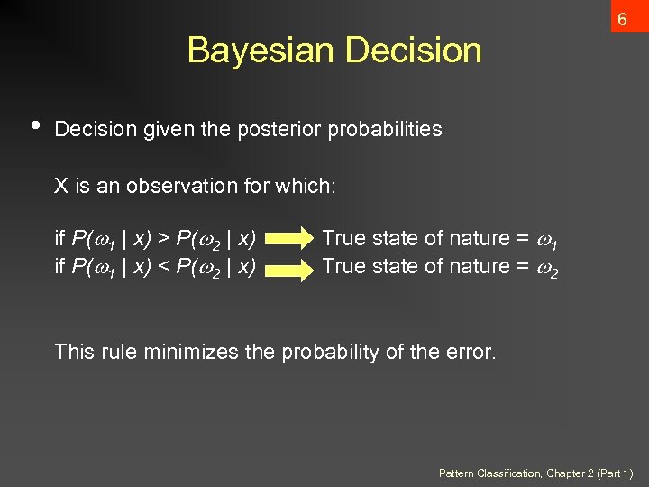6 Bayesian Decision • Decision given the posterior probabilities X is an observation for which: if P( 1 | x) > P( 2 | x) if P( 1 | x) < P( 2 | x) True state of nature = 1 True state of nature = 2 This rule minimizes the probability of the error. Pattern Classification, Chapter 2 (Part 1)

Bayesian Decision Theory – Generalization 7 • Use of more than one feature • Use more than two states of nature • Allowing actions and not only decide on the state of • nature Introduce a loss of function which is more general than the probability of error Pattern Classification, Chapter 2 (Part 1)

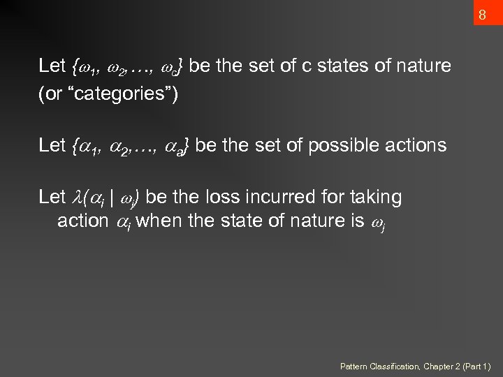8 Let { 1, 2, …, c} be the set of c states of nature (or “categories”) Let { 1, 2, …, a} be the set of possible actions Let ( i | j) be the loss incurred for taking action i when the state of nature is j Pattern Classification, Chapter 2 (Part 1)

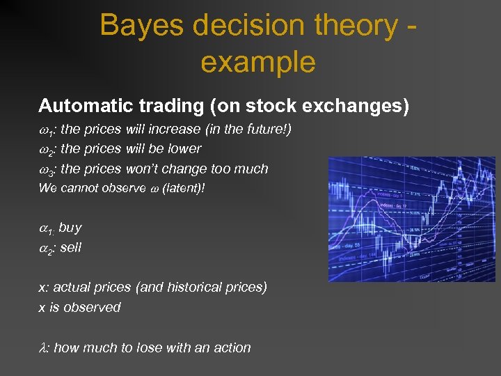Bayes decision theory example Automatic trading (on stock exchanges) 1: the prices will increase (in the future!) 2: the prices will be lower 3: the prices won’t change too much We cannot observe (latent)! 1: buy 2: sell x: actual prices (and historical prices) x is observed : how much to lose with an action

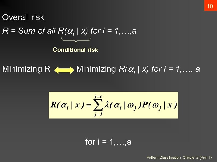10 Overall risk R = Sum of all R( i | x) for i = 1, …, a Conditional risk Minimizing R( i | x) for i = 1, …, a Pattern Classification, Chapter 2 (Part 1)

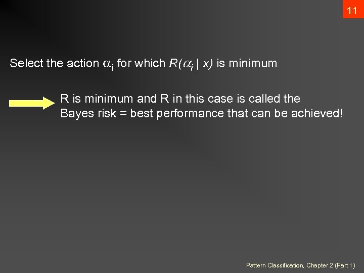11 Select the action i for which R( i | x) is minimum R is minimum and R in this case is called the Bayes risk = best performance that can be achieved! Pattern Classification, Chapter 2 (Part 1)

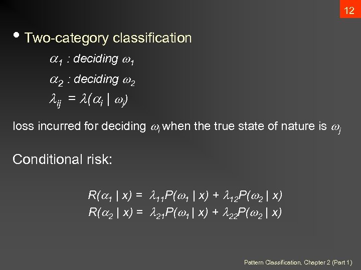12 • Two-category classification 1 : deciding 1 2 : deciding 2 ij = ( i | j) loss incurred for deciding i when the true state of nature is j Conditional risk: R( 1 | x) = 11 P( 1 | x) + 12 P( 2 | x) R( 2 | x) = 21 P( 1 | x) + 22 P( 2 | x) Pattern Classification, Chapter 2 (Part 1)

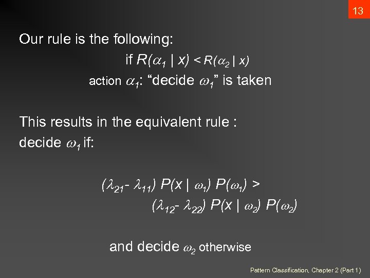13 Our rule is the following: if R( 1 | x) < R( 2 | x) action 1: “decide 1” is taken This results in the equivalent rule : decide 1 if: ( 21 - 11) P(x | 1) P( 1) > ( 12 - 22) P(x | 2) P( 2) and decide 2 otherwise Pattern Classification, Chapter 2 (Part 1)

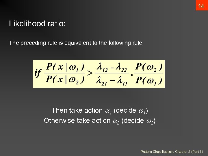14 Likelihood ratio: The preceding rule is equivalent to the following rule: Then take action 1 (decide 1) Otherwise take action 2 (decide 2) Pattern Classification, Chapter 2 (Part 1)

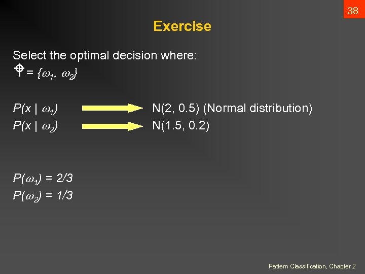
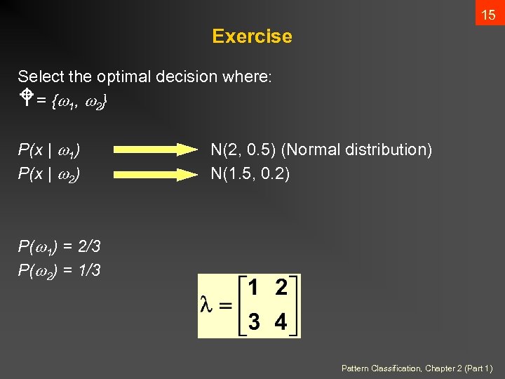15 Exercise Select the optimal decision where: W = { 1 , 2 } P(x | 1) P(x | 2) N(2, 0. 5) (Normal distribution) N(1. 5, 0. 2) P( 1) = 2/3 P( 2) = 1/3 Pattern Classification, Chapter 2 (Part 1)

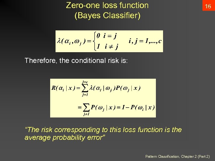Zero-one loss function (Bayes Classifier) 16 Therefore, the conditional risk is: “The risk corresponding to this loss function is the average probability error” Pattern Classification, Chapter 2 (Part 2)

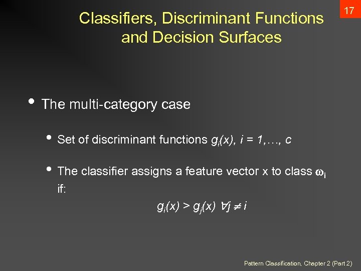Classifiers, Discriminant Functions and Decision Surfaces 17 • The multi-category case • Set of discriminant functions gi(x), i = 1, …, c • The classifier assigns a feature vector x to class i if: gi(x) > gj(x) j i Pattern Classification, Chapter 2 (Part 2)

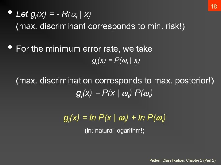18 • Let gi(x) = - R( i | x) (max. discriminant corresponds to min. risk!) • For the minimum error rate, we take gi(x) = P( i | x) (max. discrimination corresponds to max. posterior!) gi(x) P(x | i) P( i) gi(x) = ln P(x | i) + ln P( i) (ln: natural logarithm!) Pattern Classification, Chapter 2 (Part 2)

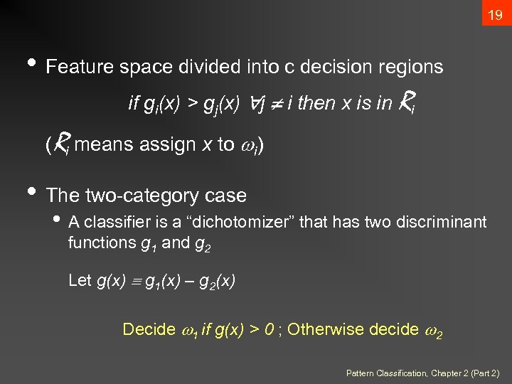19 • Feature space divided into c decision regions if gi(x) > gj(x) j i then x is in Ri (Ri means assign x to i) • The two-category case • A classifier is a “dichotomizer” that has two discriminant functions g 1 and g 2 Let g(x) g 1(x) – g 2(x) Decide 1 if g(x) > 0 ; Otherwise decide 2 Pattern Classification, Chapter 2 (Part 2)

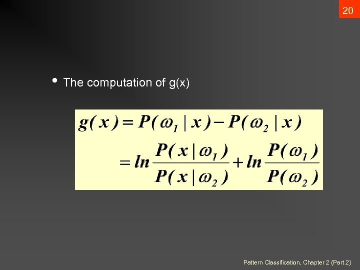20 • The computation of g(x) Pattern Classification, Chapter 2 (Part 2)

21 Discriminant functions of the Bayes Classifier with Normal Density Pattern Classification, Chapter 2 (Part 1)

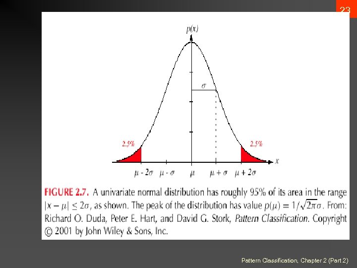
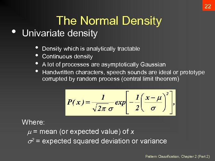22 • The Normal Density Univariate density • • Density which is analytically tractable Continuous density A lot of processes are asymptotically Gaussian Handwritten characters, speech sounds are ideal or prototype corrupted by random process (central limit theorem) Where: = mean (or expected value) of x 2 = expected squared deviation or variance Pattern Classification, Chapter 2 (Part 2)

23 Pattern Classification, Chapter 2 (Part 2)

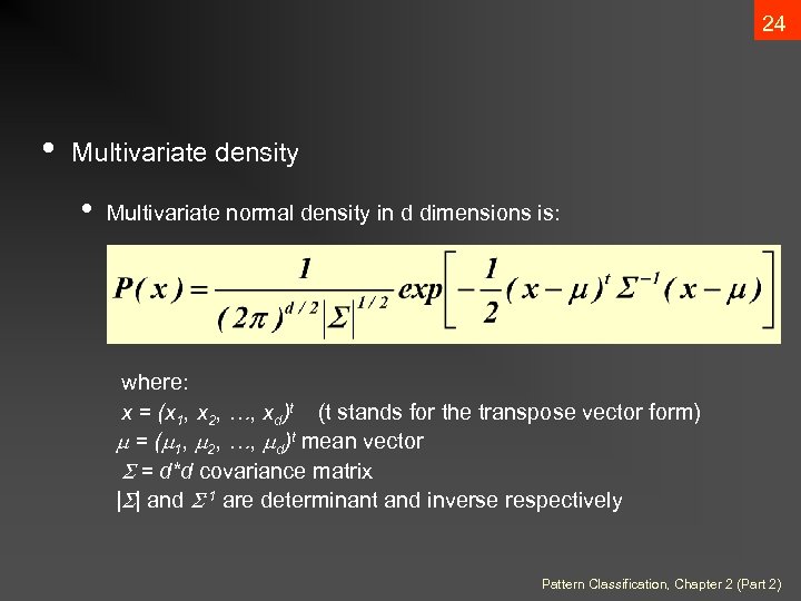24 • Multivariate density • Multivariate normal density in d dimensions is: where: x = (x 1, x 2, …, xd)t (t stands for the transpose vector form) = ( 1, 2, …, d)t mean vector = d*d covariance matrix | | and -1 are determinant and inverse respectively Pattern Classification, Chapter 2 (Part 2)

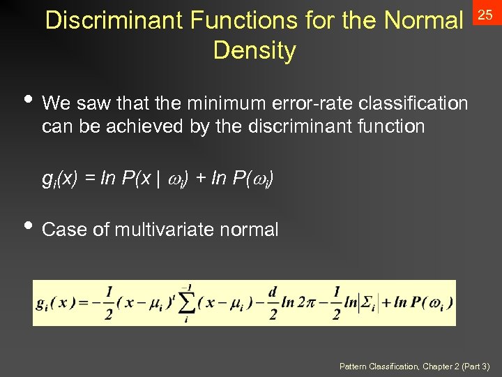Discriminant Functions for the Normal Density 25 • We saw that the minimum error-rate classification can be achieved by the discriminant function gi(x) = ln P(x | i) + ln P( i) • Case of multivariate normal Pattern Classification, Chapter 2 (Part 3)

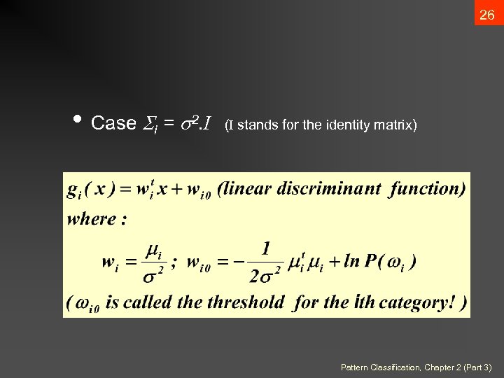26 • Case i = 2. I (I stands for the identity matrix) Pattern Classification, Chapter 2 (Part 3)

27 • A classifier that uses linear discriminant functions is called “a linear machine” • The decision surfaces for a linear machine are pieces of hyperplanes defined by: gi(x) = gj(x) Pattern Classification, Chapter 2 (Part 3)

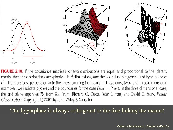28 The hyperplane is always orthogonal to the linking the means! Pattern Classification, Chapter 2 (Part 3)

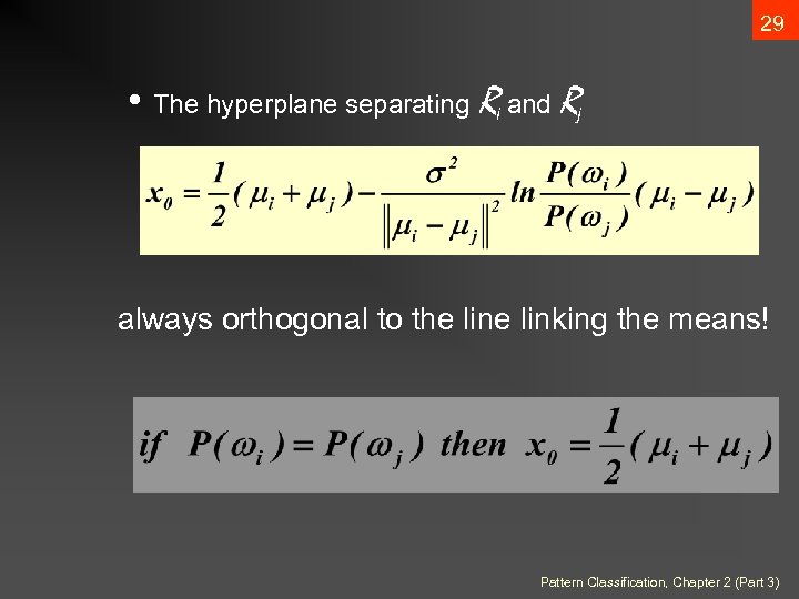29 • The hyperplane separating Ri and Rj always orthogonal to the linking the means! Pattern Classification, Chapter 2 (Part 3)

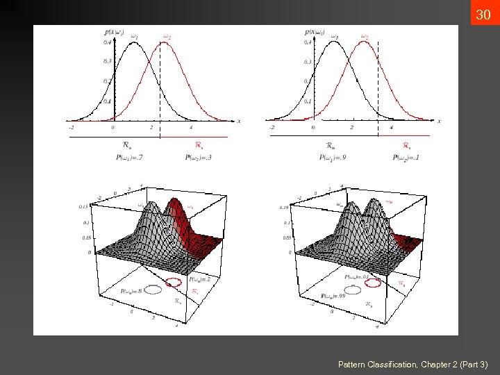30 Pattern Classification, Chapter 2 (Part 3)

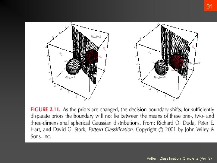31 Pattern Classification, Chapter 2 (Part 3)

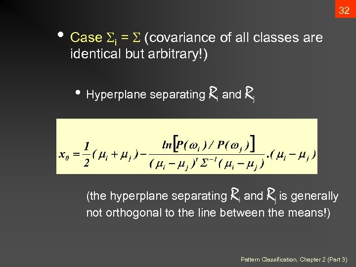32 • Case i = (covariance of all classes are identical but arbitrary!) • Hyperplane separating Ri and Rj (the hyperplane separating Ri and Rj is generally not orthogonal to the line between the means!) Pattern Classification, Chapter 2 (Part 3)

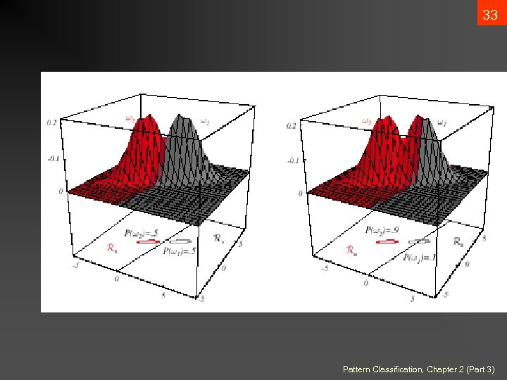33 Pattern Classification, Chapter 2 (Part 3)

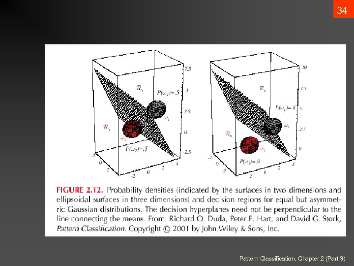34 Pattern Classification, Chapter 2 (Part 3)

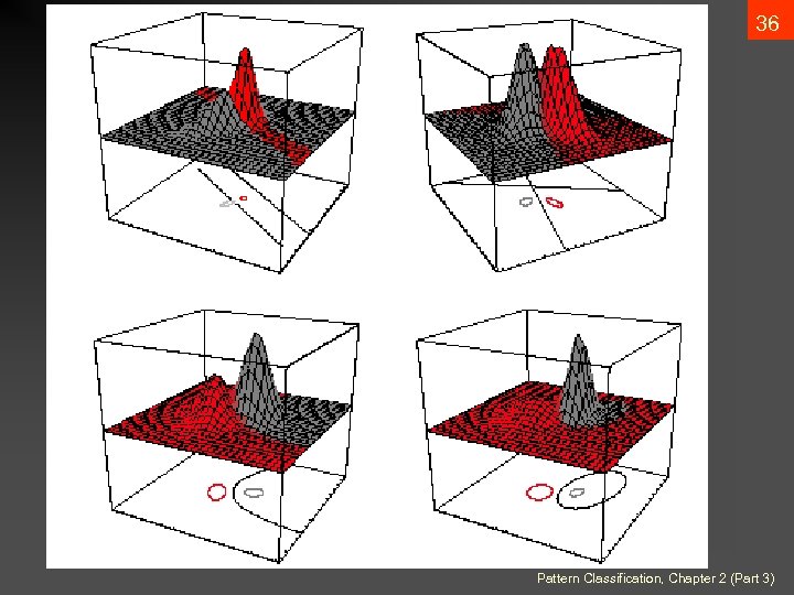
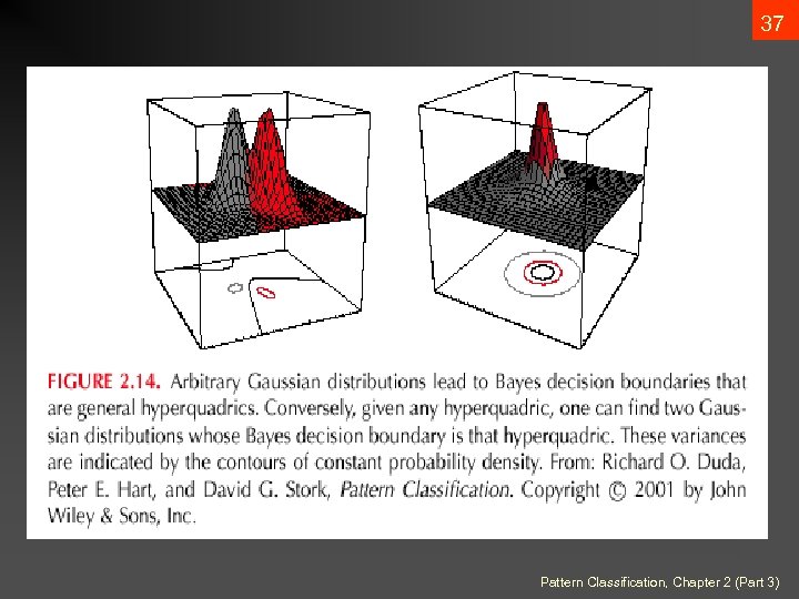
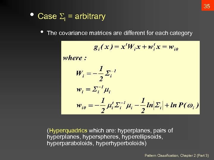35 • Case i = arbitrary • The covariance matrices are different for each category (Hyperquadrics which are: hyperplanes, pairs of hyperplanes, hyperspheres, hyperellipsoids, hyperparaboloids, hyperboloids) Pattern Classification, Chapter 2 (Part 3)

36 Pattern Classification, Chapter 2 (Part 3)

37 Pattern Classification, Chapter 2 (Part 3)

38 Exercise Select the optimal decision where: W = { 1 , 2 } P(x | 1) P(x | 2) N(2, 0. 5) (Normal distribution) N(1. 5, 0. 2) P( 1) = 2/3 P( 2) = 1/3 Pattern Classification, Chapter 2

39 Parameter estimation Pattern Classification, Chapter 3

• Data availability in a Bayesian framework • We could design an optimal classifier if we knew: • • P( i) (priors) P(x | i) (class-conditional densities) Unfortunately, we rarely have this complete information! • Design a classifier from a training sample • No problem with prior estimation • Samples are often too small for class-conditional estimation (large dimension of feature space!) 1

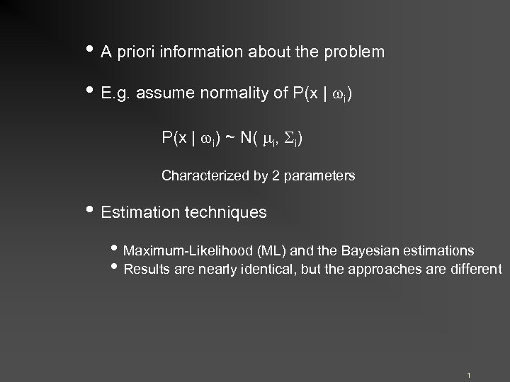• A priori information about the problem • E. g. assume normality of P(x | i) ~ N( i, i) Characterized by 2 parameters • Estimation techniques • Maximum-Likelihood (ML) and the Bayesian estimations • Results are nearly identical, but the approaches are different 1

• Parameters in ML estimation are fixed but unknown! • Best parameters are obtained by maximizing the probability of obtaining the samples observed • Bayesian methods view the parameters as random variables having some known distribution • In either approach, we use P( i | x) for our classification rule! 1

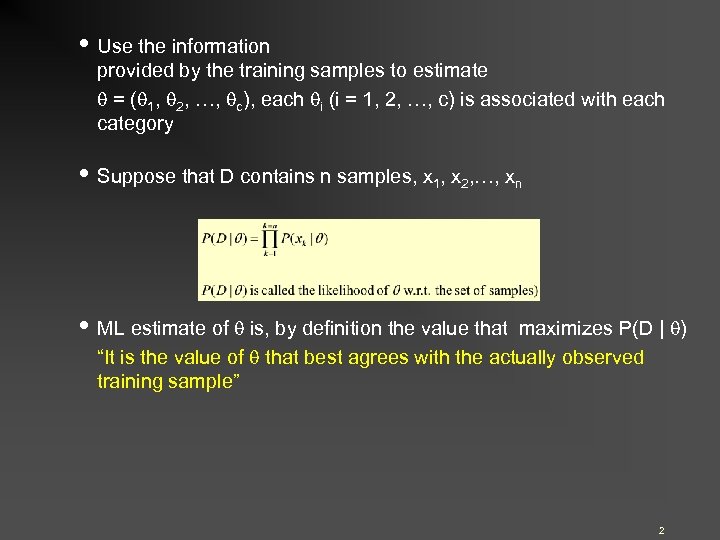• Use the information provided by the training samples to estimate = ( 1, 2, …, c), each i (i = 1, 2, …, c) is associated with each category • Suppose that D contains n samples, x 1, x 2, …, xn • ML estimate of is, by definition the value that maximizes P(D | ) “It is the value of that best agrees with the actually observed training sample” 2

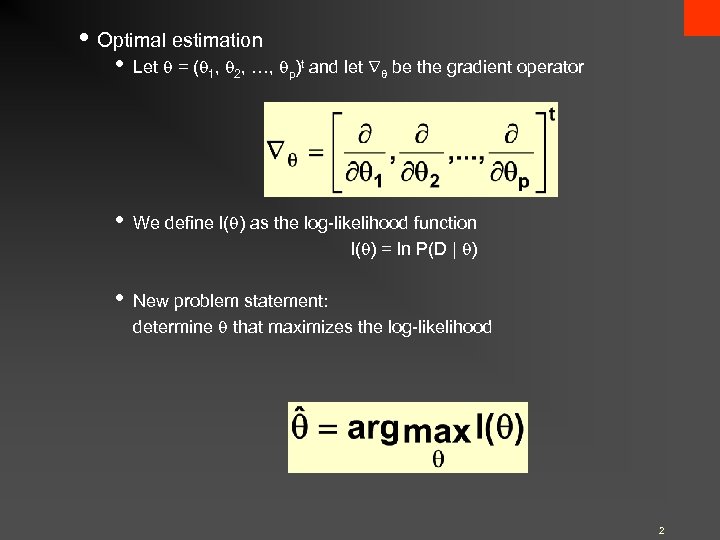• Optimal estimation • Let = ( 1, 2, …, p)t and let be the gradient operator • We define l( ) as the log-likelihood function l( ) = ln P(D | ) • New problem statement: determine that maximizes the log-likelihood 2

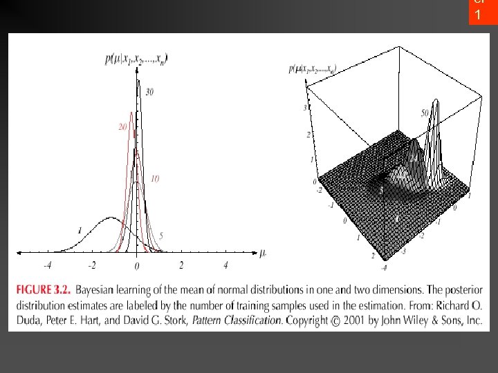
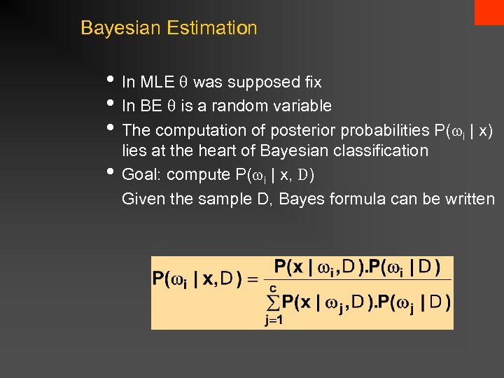Bayesian Estimation • In MLE was supposed fix • In BE is a random variable • The computation of posterior probabilities P( i | x) • lies at the heart of Bayesian classification Goal: compute P( i | x, D) Given the sample D, Bayes formula can be written

er 1

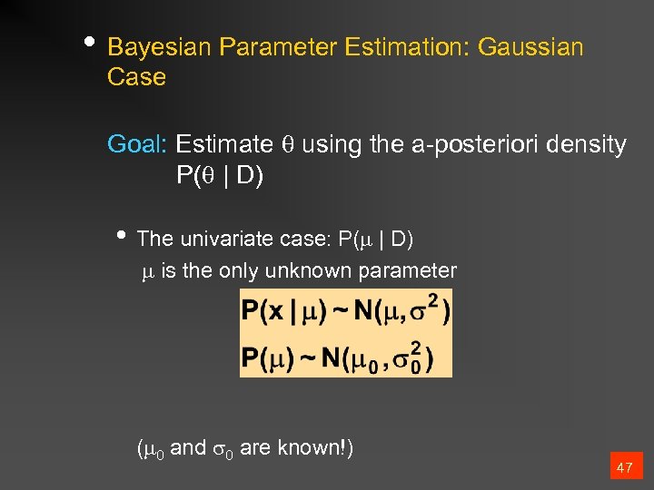• Bayesian Parameter Estimation: Gaussian Case Goal: Estimate using the a-posteriori density P( | D) • The univariate case: P( | D) is the only unknown parameter ( 0 and 0 are known!) 47

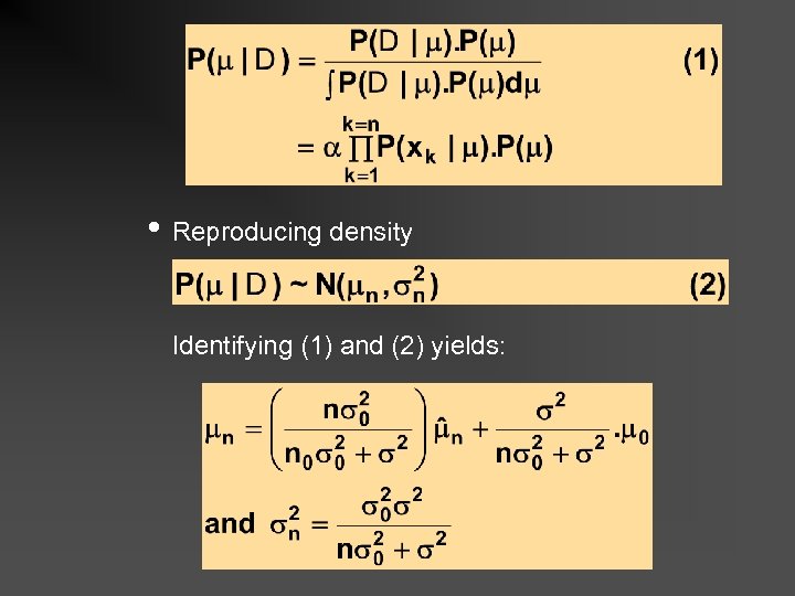• Reproducing density Identifying (1) and (2) yields:

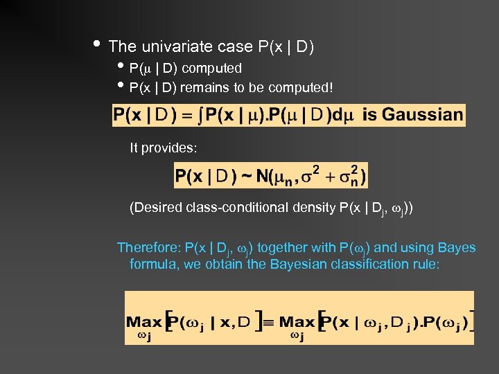• The univariate case P(x | D) • P( | D) computed • P(x | D) remains to be computed! It provides: (Desired class-conditional density P(x | Dj, j)) Therefore: P(x | Dj, j) together with P( j) and using Bayes formula, we obtain the Bayesian classification rule:

• Bayesian Parameter Estimation: General Theory • P(x | D) computation can be applied to any situation in which the unknown density can be parametrized: the basic assumptions are: • The form of P(x | ) is assumed known, but the value of • • is not known exactly Our knowledge about is assumed to be contained in a known prior density P( ) The rest of our knowledge is contained in a set D of n random variables x 1, x 2, …, xn that follows P(x) 5

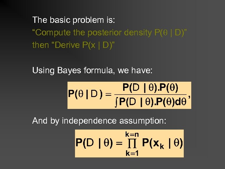The basic problem is: “Compute the posterior density P( | D)” then “Derive P(x | D)” Using Bayes formula, we have: And by independence assumption:

52 MLE vs. Bayes estimation • If n→∞ they are equal! • MLE • Simple and fast (convex optimisation vs. numerical integration) • Bayes estimation • We can express our uncertainty by P( )

Sumamry • Bayes decision theory General framework for probabilistic decision making • Bayes classifier Classification is a special decision making ( 1 : choose 1) • Zero-one loss function l can be omitted • Bayes classifier with zero-one loss with Normal Density

Summary • Parameter estimation • General procedures for densities’ parameter estimation based on a sample (it can be applied beyond Bayes classifier) • Bayesian Machine learning: the marrige of Bayesian Decision Theory and Parameter estimation from a training sample