PAST PRESENT AND FUTURE OF EARTHQUAKE ANALYSIS OF

PAST, PRESENT AND FUTURE OF EARTHQUAKE ANALYSIS OF STRUCTURES By Ed Wilson Draft dated 8/15/14 September 22 and 24 2014 SEAONC Lectures http: //edwilson. org/History/Slides/Past%20 Present%20 Future%202014. ppt

1964 Gene’s Comment – a true story. Ed developed a new program for the Analysis of Complex Rockets Ed talks to Gene -----Two weeks later Gene calls Ed -----Ed goes to see Gene ----The next day, Gene calls Ed and tells him “Ed, why did you not tell me about this program. It is the greatest program I ever used. ”

Summary of Lecture Topics 1. Fundamental Principles of Mechanics and Nature 2. Example of the Present Problem – Caltrans Criteria 3. The Response Spectrum Method 4. Demand Capacity Calculations 5. Speed of Computers– The Last Fifty Years 6. Terms I do not Understand 7. The Load Dependant Ritz Vectors - LDR Vectors 8. The Fast Nonlinear Analysis Method – FNA Method 9. Recommendations edwilson. org 10. Questions ed-wilson 1@juno. com

Fundamental Equations of Structural Analysis 1. Equilibrium - Including Inertia Forces - Must be Satisfied 2. Material Properties or Stress / Strain or Force / Deformation 3. Displacement Compatibility Or Equations or Geometry Methods of Analysis 1. Force – Good for approximate hand methods 2. Displacement - 99 % of programs use this method 3. Mixed - Beam Ex. Plane Sections & V = d. M/dz Check Conservation of Energy

My First Earthquake Engineering Paper October 1 -5 1962

THE PRESENT SAB Meeting on August 28, 2013 Comments on the Response Spectrum Analysis Method As Used in the CALTRANS SEISMIC DESIGN CRITERIA

Topics 1. Why do most Engineers have Trouble with Dynamics? Taught by people who love math – No physical examples 2 Who invented the Response Spectrum Method? Ray Clough and I did ? – by putting it into my computer program 3 Application by Cal. Trans to “Ordinary Standard Structures” Why 30 ? Why reference to Transverse & Longitudinal directions 4 Physical behavior of Skew Bridges – Failure Mode 5 Equal Displacement Rule? 6 Quote from George W. Housner

Who Developed the Approximate Response Spectrum Method of Seismic Analysis of Bridges and other Structures? 1. Fifty years ago there were only digital acceleration records for 3 earthquakes. 2. Building codes gave design spectra for a one degree of freedom systems with no guidance of how to combine the response of of the higher modes. 3. At the suggestion of Ray Clough, I programmed the square root of the sum of the square of the modal values for displacements and member forces. However, I required the user to manually combine the results from the two orthogonal spectra. Users demanded that I modify my programs to automatically combine the two directions. I refused because there was no theoretical justification. 4. The user then modify my programs by using the 100%+30% or 100%+40% rules. 5. Starting in 1981 Der Kiureghian and I published papers showing that the CQC method should be used for combining modal responses for each spectrum and the two orthogonal spectra be combined by the SRSS method. 6. We now have Thousands or of 3 D earthquake records from hundred of seismic events. Therefore, why not use Nonlinear Time-History Analyses that SATISFIES FORCE EQUILIBREUM.

Torsion or Mode 1, 2 or Mode 3

Nonlinear Failure Mode For Skew Bridges F(t) Abutment Force Acting on Bridge Tensional Failure u(t) Contact at Right Abutment u(t) Tensional Failure F(t) Abutment Force Acting on Bridge Contact at Left Abutment

Possible Torsional Failure Mode Design Joint Connectors for Joint Shear Forces?

Use a Global Modal for all Analyses

Seismic Analysis Advice by Ed Wilson 1. All Bridges are Three-Dimensional and their Dynamic Behavior is governed by the Mass and Stiffness Properties of the structure. The Longitudinal and Transverse directions are geometric properties. All Structures have Torsional Modes of Vibrations. 2. The Response Spectrum Analysis Method is a very approximate method of seismic analysis which only produces positive values of displacements and member forces which are not in equilibrium. Demand / Capacity Ratios have Very Large Errors 3. A structural engineer may take several days to prepare and verify a linear SAP 2000 model of an Ordinary Standard Bridge. It would take less than a day to add Nonlinear Gap Elements to model the joints. If a family of 3 D earthquake motions are specified, the program will automatically summarize the maximum demand-capacity ratios and the time they occur in a few minutes of computer time.

Convince Yourself with a simple test problem 1. Select an existing Sap 2000 model of a Ordinary Standard Bridge with several different spans – both straight and curved. 2. Select one earthquake ground acceleration record to be used as the input loading which is approximately 20 seconds long. 3. Create a spectrum from the selected earthquake ground acceleration record. 4. Using a number of modes that captures a least 90 percent of the mass in all three directions. 5. At a 45 degree angle, Run a Linear Time History Analysis and a Response Spectrum Analysis. 6. Compare Demand Capacity Ratios for both SAP 2000 analysis for all members. 7. You decide if the Approximate RSA results are in good agreement with the Linear time History Results.

Educational Priorities of an Old Professor on Seismic Analysis of Structures Convince Engineers that the Response Spectrum Method Produces very Poor Results 1. Method is only exact for single degree of freedom systems 2. It produces only positive numbers for Displacements and Member Forces. 3. Results are maximum probable values and occur at an “Unknown Time” 4. Short and Long Duration earthquakes are treated the same using “Design Spectra” 5. Demand/Capacity Ratios are always “Over Conservative” for most Members. 6. The Engineer does not gain insight into the “Dynamic Behavior of the Structure” Results are not in equilibrium. More modes and 3 D analysis will cause more errors. 7. Nonlinear Spectra Analysis is “Smoke and Mirrors” – Forget it

Convince Engineers that it is easy to conduct “Linear Dynamic Response Analysis” It is a simple extension of Static Analysis – just add mass and time dependent loads 1. Static and Dynamic Equilibrium is satisfied at all points in time if all modes are included 2. Errors in the results can be estimated automatically if modes are truncated 3. Time-dependent plots and animation are impressive and fun to produce 4. Capacity/Demand Ratios are accurate and a function of time – summarized by program. 5. Engineers can gain great insight into the dynamic response of the structure and may help in the redesign of the structural system.

Terminology commonly used in nonlinear analysis that do not have a unique definition 1. Equal Displacement Rule – can you prove it? 2. Pushover Analysis 3. Equivalent Linear Damping 4. Equivalent Static Analysis 5. Nonlinear Spectrum Analysis 6. Onerous Response History Analysis

Equal Displacement Rule In 1960 Veletsos and Newmark proposed in a paper presented at the 2 nd WCEE For a one DOF System, subjected to the El Centro Earthquake, the Maximum Displacement was approximately the same for both linear and nonlinear analyses. In 1965 Clough and Wilson, at the 3 rd WCEE, proved the Equal Displacement Rule did not apply to multi DOF structures. http: //edwilson. org/History/Pushover. pdf

1965 Professor Clough’s Comment. “If tall buildings are designed for elastic column behavior and restrict the nonlinear bending behavior to the girders, it appears the danger of total collapse of the building is reduced. ” This indicates the strong-column and week beam design is the one of the first statements on Performance Based Design

The Response Spectrum Method Basic Assumptions I do not know who first called it a “response spectrum, ” but unfortunate the term leads people to think that the characterize the building’s motion, rather than the ground’s motion. George W. Housner EERI Oral History, 1996

Typical Earthquake Ground Acceleration – percent of gravity

Integration will produce Earthquake Ground Displacement – inches These real Eq. Displacement can be used as Computer Input

Relative Displacement Spectrum for a unit mass with different periods 1. These displacements Ymax are maximum (+ or -) values versus period for a structure or mode. 2. Note: we do not know the time these maximum took place. Pseudo Acceleration Spectrum Note: S = w 2 Ymax has the same properties as the Displacement Spectrum. Therefore, how can anyone justify combining values, which occur at different times, and expect to obtain accurate results. CASE CLOSED

General Horizontal Response Spectrum from ASCE 41 - 06

Where did the Hat go - on the Response Spectrum ? As I Recall -------

Demand-Capacity Ratios The Demand-Capacity ratio for a linear elastic, compression member is given by an equation of the following general form: If the axial force and the two moments are a function of time, the Demand-Capacity ratio will be a function of time and a smart computer program will produce R(max) and the time it occurred. A smart engineer will hand check several of these values.

RSM Demand-Capacity Ratios If the axial force and the two moments are produced by the Response Spectrum Method the Demand-Capacity ratio may be computed by an equation of the following general form: A smart computer program can compute this Demand. Capacity Ratio. However, only an idiot would believe it.

SPEED and COST of COMPUTERS 1957 to 2014 to the Cloud You can now buy a very powerful small computer for less than $1, 000 However, it may cost you several thousand dollars of your time to learn how to use all the new options. If it has a new operating system

1957 My First Computer in Cory Hall IBM 701 Vacuum Tube Digital Computer Could solve 40 equations in 30 minutes

1981 My First Computer Assembled at Home Paid $6000 for a 8 bit CPM Operating System with FORTRAN. Used it to move programs from the CDC 6400 to the VAX on Campus. Developed a new program called SAP 80 without using any Statements from previous versions of SAP. After two years, system became obsolete when IBM released DOS with a floating point chip. In 1984, CSI developed Graphics and Design Post-Processor and started distribution of the Professional Version of Sap 80

Floating-Point Speeds of Computer Systems Definition of one Operation A = B + C*D Operations Per Second 64 bits - REAL*8 Year Computer or CPU Relative Speed 1962 CDC-6400 50, 000 1 1964 CDC-6600 100, 000 2 1974 CRAY-1 3, 000 60 1981 IBM-3090 20, 000 400 1981 CRAY-XMP 40, 000 800 1994 Pentium-90 3, 500, 000 70 1995 Pentium-133 5, 200, 000 104 1995 DEC-5000 upgrade 14, 000 280 1998 Pentium II - 333 37, 500, 000 750 1999 Pentium III - 450 69, 000 1, 380

Cost of Personal Computer Systems YEAR CPU Speed MHz Operations Per Second Relative Speed 1980 8080 4 200 1 $6, 000 1984 8087 10 13, 000 65 $2, 500 1988 80387 20 93, 000 465 $8, 000 1991 80486 33 605, 000 3, 025 $10, 000 1994 80486 66 1, 210, 000 6, 050 $5, 000 1996 Pentium 233 10, 300, 000 52, 000 $4, 000 1997 Pentium II 233 11, 500, 000 58, 000 $3, 000 1998 Pentium II 333 37, 500, 000 198, 000 $2, 500 1999 Pentium III 450 69, 000 345, 000 $1, 500 2003 Pentium IV 2000 220, 000 1. 100, 000 $2. 000 2006 AMD - Athlon 2000 440, 000 2, 200, 000 $950 COST

Year Computer or CPU Cost Operations Per Second Relative Speed 1962 CDC-6400 $1, 000 50, 000 1 1974 CRAY-1 $4, 000 3, 000 60 1981 VAX or Prime $100, 000 1994 Pentium-90 $5, 000 4, 000 1999 Intel Pentium III-450 $1, 500 69, 000 2006 AMD 64 Laptop $2, 000 400, 000 2009 Min Laptop $300 200, 000 2. 4 GHz Intel Core i 3 64 bit Win 7 Laptop $1, 000 1. 35 Billion Intel Fortran 27, 000 2. 80 GHz 2 Quad Core 64 bit Win 7 $1, 000 2. 80 Billion Parallelized Fortran 56, 000 2013 2 70 1, 380 8, 000 4, 000 The cost of one operation has been reduced by 56, 000 in the last 50 years

Computer Cost versus Engineer’s Monthly Salary $1, 000 c/s = 0. 10 $10, 000 $1, 000 1963 Time 2013

Fast Nonlinear Analysis With Emphasis On Earthquake Engineering BY Ed Wilson Professor Emeritus of Civil Engineering University of California, Berkeley edwilson. org May 25, 2006

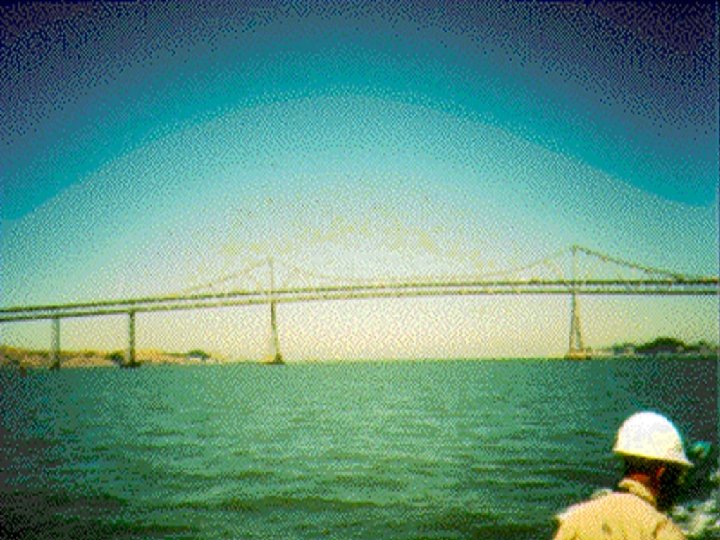
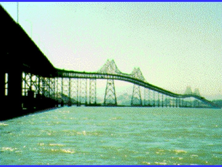
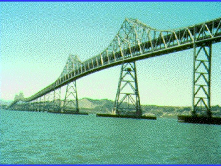
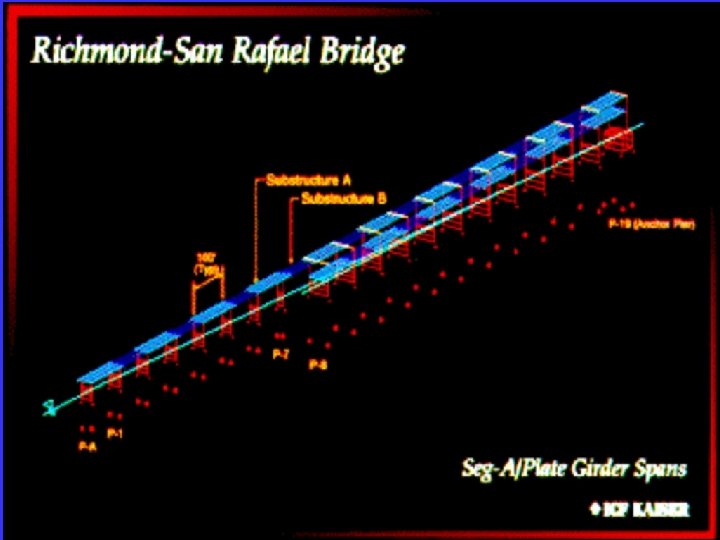
Summary Of Presentation 1. History of the Finite Element Method 2. History Of The Development of SAP 3. Computer Hardware Developments 4. Methods For Linear and Nonlinear Analysis 5. Generation And Use Of LDR Vectors and Fast Nonlinear Analysis - FNA Method 6. Example Of Parallel Engineering Analysis of the Richmond - San Rafael Bridge

From The Foreword Of The First SAP Manual "The slang name S A P was selected to remind the user that this program, like all programs, lacks intelligence. It is the responsibility of the engineer to idealize the structure correctly and assume responsibility for the results. ” Ed Wilson 1970

The SAP Series of Programs 1969 - 70 SAP Used Static Loads to Generate Ritz Vectors 1971 - 72 Solid-Sap Rewritten by Ed Wilson 1972 -73 SAP IV Subspace Iteration – Dr. Jűgen 1973 – 74 NON SAP New Program – The Start of ADINA 1979 – 80 SAP 80 New Linear Program for Personal Computers Bathe Lost All Research and Development Funding 1983 – 1987 SAP 80 CSI added Pre and Post Processing 1987 - 1990 SAP 90 Significant Modification and Documentation 1997 – Present SAP 2000 Nonlinear Elements – More Options – With Windows Interface

Load-Dependent Ritz Vectors LDR Vectors – 1980 - 2000

MOTAVATION – 3 D Reactor on Soft Foundation Dynamic Analysis - 1979 by Bechtel using SAP IV 200 Exact Eigenvalues were Calculated and all of the Modes were in the foundation – No Stresses in the Reactor. The cost for the analysis on the CLAY Computer was $10, 000 3 D Concrete Reactor 3 D Soft Soil Elements 360 degrees

DYNAMIC EQUILIBRIUM EQUATIONS M a + C v + K u = F(t) a v u M C K F(t) = = = = Node Accelerations Node Velocities Node Displacements Node Mass Matrix Damping Matrix Stiffness Matrix Time-Dependent Forces

PROBLEM TO BE SOLVED Ma + Cv+ Ku = fi g(t)i = - Mx a x - M y a y - Mz a z For 3 D Earthquake Loading THE OBJECTIVE OF THE ANALYSIS IS TO SOLVE FOR ACCURATE DISPLACEMENTS and MEMBER FORCES

METHODS OF DYNAMIC ANALYSIS For Both Linear and Nonlinear Systems ÷ STEP BY STEP INTEGRATION - 0, dt, 2 dt. . . N dt USE OF MODE SUPERPOSITION WITH EIGEN OR LOAD-DEPENDENT RITZ VECTORS FOR FNA For Linear Systems Only TRANSFORMATION TO THE FREQUENCY ÷ DOMAIN and FFT METHODS RESPONSE SPECTRUM METHOD - CQC - SRSS

STEP BY STEP SOLUTION METHOD 1. Form Effective Stiffness Matrix 2. Solve Set Of Dynamic Equilibrium Equations For Displacements At Each Time Step 3. For Non Linear Problems Calculate Member Forces For Each Time Step and Iterate for Equilibrium - Brute Force Method

MODE SUPERPOSITION METHOD 1. Generate Orthogonal Dependent Vectors And Frequencies 2. Form Uncoupled Modal Equations And Solve Using An Exact Method For Each Time Increment. 3. Recover Node Displacements As a Function of Time 4. Calculate Member Forces As a Function of Time

GENERATION DEPENDENT LOAD VECTORS OF RITZ 1. Approximately Three Times Faster Than The Calculation Of Exact Eigenvectors 2. Results In Improved Accuracy Using A Smaller Number Of LDR Vectors 3. Computer Storage Requirements Reduced 4. Can Be Used For Nonlinear Analysis To Capture Local Static Response

STEP 1. INITIAL CALCULATION A. TRIANGULARIZE STIFFNESS MATRIX B. DUE TO A BLOCK OF STATIC LOAD VECTORS, f, SOLVE FOR A BLOCK OF DISPLACEMENTS, u, Ku=f C. MAKE FORM u STIFFNESS AND MASS ORTHOGONAL TO FIRST BLOCK OF LDL VECTORS V 1 T M V 1 = I

STEP 2. VECTOR GENERATION i = 2. . N Blocks A. Solve for Block of Vectors, K Xi = M Vi-1 B. Make Vector Block, Xi , Stiffness and Mass Orthogonal - Yi C. Use Modified Gram-Schmidt, Twice, to Make Block of Vectors, Yi , Orthogonal to all Previously Calculated Vectors - Vi

STEP 3. MAKE VECTORS STIFFNESS ORTHOGONAL A. SOLVE Nb x Nb Eigenvalue Problem [ V T K V ] Z = [ w 2 ] Z B. CALCULATE MASS AND STIFFNESS ORTHOGONAL LDR VECTORS VR = V Z =

DYNAMIC RESPONSE OF BEAM 100 pounds 10 AT 12" = 120" FORCE = Step Function TIME

MAXIMUM DISPLACEMENT Number of Vectors Eigen Vectors Load Dependent Vectors 1 0. 004572 (-2. 41) 0. 004726 (+0. 88) 2 0. 004572 (-2. 41) 0. 004591 ( -2. 00) 3 0. 004664 (-0. 46) 0. 004689 (+0. 08) 4 0. 004664 (-0. 46) 0. 004685 (+0. 06) 5 0. 004681 (-0. 08) 0. 004685 ( 0. 00) 7 0. 004683 (-0. 04) 9 0. 004685 (0. 00) ( Error in Percent)

MAXIMUM MOMENT Number of Vectors Eigen Vectors Load Dependent Vectors 1 4178 ( - 22. 8 %) 5907 ( + 9. 2 ) 2 4178 ( - 22. 8 ) 5563 ( + 2. 8 ) 3 4946 ( - 8. 5 ) 5603 ( + 3. 5 ) 4 4946 ( - 8. 5 ) 5507 ( + 1. 8) 5 5188 ( - 4. 1 ) 5411 ( 0. 0 ) 7 5304 ( -. 0 ) 9 5411 ( 0. 0 ) ( Error in Percent )

LDR Vector Summary After Over 20 Years Experience Using the LDR Vector Algorithm We Have Always Obtained More Accurate Displacements and Stresses Compared to Using the Same Number of Exact Dynamic Eigenvectors. SAP 2000 has Both Options

The Fast Nonlinear Analysis Method The FNA Method was Named in 1996 Designed for the Dynamic Analysis of Structures with a Limited Number of Predefined Nonlinear Elements

FAST NONLINEAR ANALYSIS 1. EVALUATE LDR VECTORS WITH NONLINEAR ELEMENTS REMOVED AND DUMMY ELEMENTS ADDED FOR STABILITY 2. SOLVE ALL MODAL EQUATIONS WITH NONLINEAR FORCES ON THE RIGHT HAND SIDE 3. USE EXACT INTEGRATION WITHIN EACH TIME STEP 4. FORCE AND ENERGY EQUILIBRIUM ARE STATISFIED AT EACH TIME STEP BY ITERATION

BASE ISOLATION Isolators

BUILDING IMPACT ANALYSIS

FRICTION DEVICE CONCENTRATED DAMPER NONLINEAR ELEMENT

GAP ELEMENT BRIDGE DECK ABUTMENT TENSION ONLY ELEMENT

PLASTIC HINGES 2 ROTATIONAL DOF DEGRADING STIFFNESS ?

Mechanical Damper F = f (u, v, umax ) F = ku F = C v. N Mathematical Model

LINEAR VISCOUS DAMPING DOES NOT EXIST IN NORMAL STRUCTURES AND FOUNDATIONS 5 OR 10 PERCENT MODAL DAMPING VALUES ARE OFTEN USED TO JUSTIFY ENERGY DISSIPATION DUE TO NONLINEAR EFFECTS IF ENERGY DISSIPATION DEVICES ARE USED THEN 1 PERCENT MODAL DAMPING SHOULD BE USED FOR THE ELASTIC PART OF THE STRUCTURE - CHECK ENERGY PLOTS

103 FEET DIAMETER - 100 FEET HEIGHT NONLINEAR DIAGONALS BASE ISOLATION ELEVATED WATER STORAGE TANK

COMPUTER MODEL 92 NODES 103 ELASTIC FRAME ELEMENTS 56 NONLINEAR DIAGONAL ELEMENTS 600 TIME STEPS @ 0. 02 Seconds

COMPUTER TIME REQUIREMENTS PROGRAM ANSYS INTEL 486 3 Days ANSYS CRAY 3 Hours SADSAP INTEL 486 ( B Array was 56 x 20 ) ( 4300 Minutes ) ( 180 Minutes ) (2 Minutes )

Nonlinear Equilibrium Equations

Nonlinear Equilibrium Equations

Summary Of FNA Method 1. Calculate LDR Vectors for Structure With the Nonlinear Elements Removed. 2. These Vectors Satisfy the Following Orthogonality Properties

3. The Solution Is Assumed to Be a Linear Combination of the LDR Vectors. Or, Which Is the Standard Mode Superposition Equation Remember the LDR Vectors Are a Linear Combination of the Exact Eigenvectors; Plus, the Static Displacement Vectors. No Additional Approximations Are Made.

4. A typical modal equation is uncoupled. However, the modes are coupled by the unknown nonlinear modal forces which are of the following form: 5. The deformations in the nonlinear elements can be calculated from the following displacement transformation equation:

6. Since the deformations in the nonlinear elements can be expressed in terms of the modal response by Where the size of the array is equal to the number of deformations times the number of LDR vectors. The array is calculated only once prior to the start of mode integration. THE ARRAY CAN BE STORED IN RAM

7. 7. The nonlinear element forces are calculated, for iteration i , at the end of each time step

8. Calculate error for iteration i , at the end of each time step, for the N Nonlinear elements – given Tol

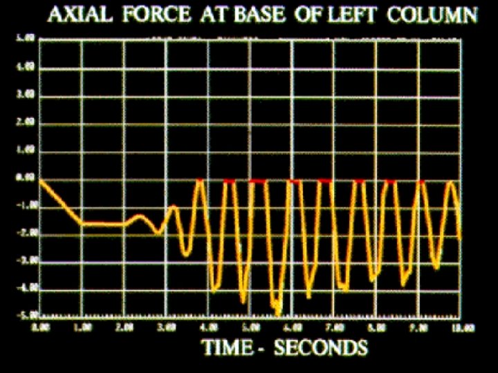
FRAME WITH UPLIFTING ALLOWED

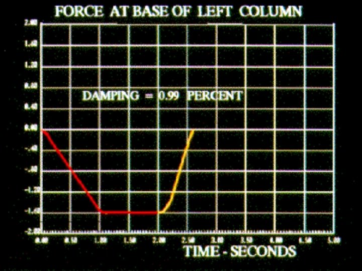
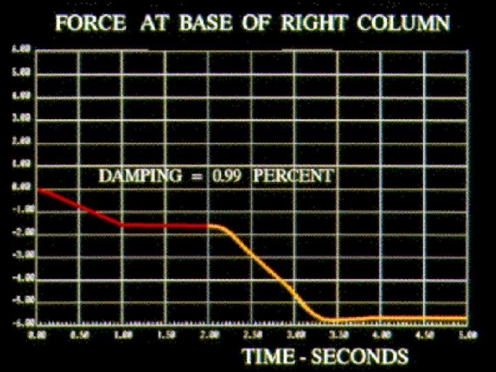
Four Static Load Conditions Are Used To Start The Generation of LDR Vectors EQ DL Left Right

NONLINEAR STATIC ANALYSIS 50 STEPS AT d. T = 0. 10 SECONDS DEAD LOAD LATERAL LOAD 0 1. 0 2. 0 3. 0 4. 0 5. 0 TIME - Seconds

Advantages Of The FNA Method 1. The Method Can Be Used For Both Static And Dynamic Nonlinear Analyses 2. The Method Is Very Efficient And Requires A Small Amount Of Additional Computer Time As Compared To Linear Analysis 2. The Method Can Easily Be Incorporated Into Existing Computer Programs For LINEAR DYNAMIC ANALYSIS.

PARALLEL ENGINEERING AND PARALLEL COMPUTERS

ONE PROCESSOR ASSIGNED TO EACH JOINT 3 2 1 1 2 3 ONE PROCESSOR ASSIGNEDTO EACH MEMBER

PARALLEL STRUCTURAL ANALYSIS DIVIDE STRUCTURE INTO "N" DOMAINS FORM ELEMENT STIFFNESS IN PARALLEL FOR "N" SUBSTRUCTURES FORM AND SOLVE EQUILIBRIUM EQ. EVALUATE ELEMENT FORCES IN PARALLEL IN "N" SUBSTRUCTURES NONLINEAR LOOP TYPICAL COMPUTER

FIRST PRACTICAL APPLICTION OF THE FNA METHOD Retrofit of the RICHMOND - SAN RAFAEL BRIDGE 1997 to 2000 Using SADSAP

S A D S A P TATIC ND YNAMIC TRUCTURAL NALYSIS ROGRAM

TYPICAL ANCHOR PIER

MULTISUPPORT ANALYSIS ( Displacements ) ANCHOR PIERS RITZ VECTOR LOAD PATTERNS

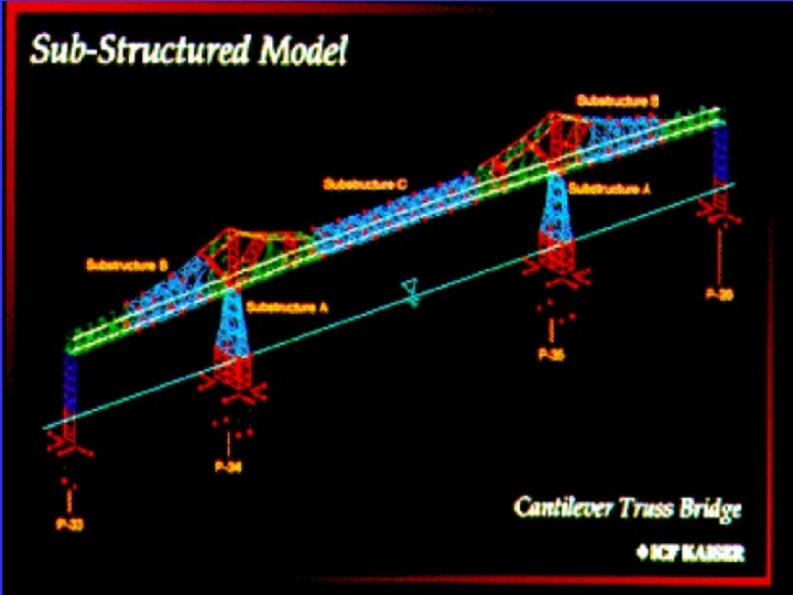
SUBSTRUCTURE PHYSICS Stiffness Matrix Size = 3 x 16 = 48 "a" MASSLESS JOINT ( Eliminated DOF ) "b" MASS POINTS and JOINT REACTIONS ( Retained DOF )

SUBSTRUCTURE STIFFNESS REDUCE IN SIZE BY LUMPING MASSES OR BY ADDING INTERNAL MODES

ADVANTAGES IN THE USE OF SUBSTRUCTURES 1. FORM OF MESH GENERATION 2. LOGICAL SUBDIVISION OF WORK 3. MANY SHORT COMPUTER RUNS 4. RERUN ONLY SUBSTRUCTURES WHICH WERE REDESIGNED 5. PARALLEL POST PROCESSING USING NETWORKING

ECCENTRICALLY BRACED FRAME

FIELD MEASUREMENTS REQUIRED TO VERIFY 1. MODELING ASSUMPTIONS 2. SOIL-STRUCTURE MODEL 3. COMPUTER PROGRAM 4. COMPUTER USER

CHECK OF RIGID DIAPHRAGM APPROXIMATION MECHANICAL VIBRATION DEVICES

FIELD MEASUREMENTS OF PERIODS AND MODE SHAPES MODE TFIELD TANALYSIS Diff. - % 1 2 3 4 5 6 7 - 1. 77 Sec. 1. 69 1. 68 0. 60 0. 59 0. 32 - 1. 78 Sec. 1. 68 0. 61 0. 59 0. 32 - 0. 5 0. 6 0. 0 0. 9 0. 8 0. 2 - 11 0. 23 0. 32 2. 3

FIRST DIAPHRAGM MODE SHAPE 15 th Period TFIELD = 0. 16 Sec.

At the Present Time Most Laptop Computers Can be directly connected to a 3 D Acceleration Seismic Box Therefore, Every Earthquake Engineer C an verify Computed Frequencies If software has been developed

Final Remark Geotechnical Engineers must produce realistic Earthquake records for use by Structural Engineers

Errors Associated with the use of Relative Displacements Compared with the use of real Physical Earthquake Displacements Classical Viscous Damping does not exist In the Real Physical World

Comparison of Relative and Absolute Displacement Seismic Analysis

Shear at Second Level Vs. Time With Zero Damping Time Step = 0. 01

Illustration of Mass-Proportional Component in Classical Damping.