a4694c3a12366a0fbe36638cac8f5fcf.ppt
- Количество слайдов: 66
Part III Probability and Probability Distributions Sullivan – Fundamentals of Statistics – 2 nd Edition – Chapter 5 Introduction – Slide 1 of 5
Chapter 5 Probability Sullivan – Fundamentals of Statistics – 2 nd Edition – Chapter 5 Introduction – Slide 2 of 5
Chapter 5 ● When we talk about probability, we are talking about a (mathematical) measure of how likely it is for some particular thing to happen ● Probability deals with chance behavior § We study outcomes, or results of experiments § Each time we conduct an experiment, we may get a different result § Probability models the short-term behavior of experiments Sullivan – Fundamentals of Statistics – 2 nd Edition – Chapter 5 Introduction – Slide 3 of 5
Chapter 5 – Section 1 ● Rule – the probability of any event must be greater than or equal to 0 and less than or equal to 1 § It does not make sense to say that there is a – 30% chance of rain § It does not make sense to say that there is a 140% chance of rain ● Note – probabilities can be written as decimals (0, 0. 3, 1. 0), or as percents (0%, 30%, 100%), or as fractions (3/10) Sullivan – Fundamentals of Statistics – 2 nd Edition – Chapter 5 Introduction – Slide 4 of 5
Chapter 5 – Section 1 ● If we do not know the probability of a certain event E, we can conduct a series of experiments to approximate it by ● This becomes a good approximation for P(E) if we have a large number of trials (the law of large numbers) Sullivan – Fundamentals of Statistics – 2 nd Edition – Chapter 5 Introduction – Slide 5 of 5
Chapter 5 – Section 1 ● Sometimes probabilities are difficult to calculate, but the experiment can be simulated on a computer ● If we simulate the experiment multiple times, then this is similar to the situation for the empirical method ● We can use Sullivan – Fundamentals of Statistics – 2 nd Edition – Chapter 5 Introduction – Slide 6 of 5
Chapter 5 – Section 1 ● Example ● We wish to determine what proportion of students at a certain school have type A blood § We perform an experiment (a simple random sample!) with 100 students § If 29 of those students have type A blood, then we would estimate that the proportion of students at this school with type A blood is 29% Sullivan – Fundamentals of Statistics – 2 nd Edition – Chapter 5 Introduction – Slide 7 of 5
Chapter 5 ● Descriptive statistics, describing and summarizing data, deals with data as it is ● Probability , modeling data, deals with data as it is predicted to be ● The combination of the two will let us do our inferential statistics techniques in Part IV Sullivan – Fundamentals of Statistics – 2 nd Edition – Chapter 5 Introduction – Slide 8 of 5
Chapter 6 Discrete Probability Distributions Sullivan – Fundamentals of Statistics – 2 nd Edition – Chapter 5 Introduction – Slide 9 of 5
Overview ● These are probability distributions that are designed to model discrete variables ● Many of the discrete probability distributions model “counts” Sullivan – Fundamentals of Statistics – 2 nd Edition – Chapter 5 Introduction – Slide 10 of 5
Chapter 6 Sections ● Sections in Chapter 6 6. 1 § 6. 2 § Discrete Random Variables The Binomial Probability Distribution Sullivan – Fundamentals of Statistics – 2 nd Edition – Chapter 5 Introduction – Slide 11 of 5
Chapter 6 Section 1 Discrete Random Variables Sullivan – Fundamentals of Statistics – 2 nd Edition – Chapter 5 Introduction – Slide 12 of 5
Chapter 6 – Section 1 ● Learning objectives 1 § 2 § 3 § 4 § 5 § 6 § Distinguish between discrete and continuous random variables Identify discrete probability distributions Construct probability histograms Compute and interpret the mean of a discrete random variable Interpret the mean of a discrete random variable as an expected value Compute the variance and standard deviation of a discrete random variable Sullivan – Fundamentals of Statistics – 2 nd Edition – Chapter 5 Introduction – Slide 13 of 5
Chapter 6 – Section 1 ● Learning objectives 1 § 2 § 3 § 4 § 5 § 6 § Distinguish between discrete and continuous random variables Identify discrete probability distributions Construct probability histograms Compute and interpret the mean of a discrete random variable Interpret the mean of a discrete random variable as an expected value Compute the variance and standard deviation of a discrete random variable Sullivan – Fundamentals of Statistics – 2 nd Edition – Chapter 5 Introduction – Slide 14 of 5
Chapter 6 – Section 1 ● A random variable is a numeric measure of the outcome of a probability experiment § Random variables reflect measurements that can change as the experiment is repeated § Random variables are denoted with capital letters, typically using X (and Y and Z …) § Values are usually written with lower case letters, typically using x (and y and z. . . ) Sullivan – Fundamentals of Statistics – 2 nd Edition – Chapter 5 Introduction – Slide 15 of 5
Chapter 6 – Section 1 ● Examples ● Tossing four coins and counting the number of heads § The number could be 0, 1, 2, 3, or 4 § The number could change when we toss another four coins ● Measuring the heights of students § The heights could change from student to student Sullivan – Fundamentals of Statistics – 2 nd Edition – Chapter 5 Introduction – Slide 16 of 5
Chapter 6 – Section 1 ● A discrete random variable is a random variable that has either a finite or a countable number of values § A finite number of values such as {0, 1, 2, 3, and 4} § A countable number of values such as {1, 2, 3, …} ● Discrete random variables are designed to model discrete variables (see section 1. 2) ● Discrete random variables are often “counts of …” Sullivan – Fundamentals of Statistics – 2 nd Edition – Chapter 5 Introduction – Slide 17 of 5
Chapter 6 – Section 1 ● An example of a discrete random variable ● The number of heads in tossing 3 coins (a finite number of possible values) § There are four possible values – 0 heads, 1 head, 2 heads, and 3 heads § A finite number of possible values – a discrete random variable § This fits our general concept that discrete random variables are often “counts of …” Sullivan – Fundamentals of Statistics – 2 nd Edition – Chapter 5 Introduction – Slide 18 of 5
Chapter 6 – Section 1 ● Other examples of discrete random variables ● The possible rolls when rolling a pair of dice § A finite number of possible pairs, ranging from (1, 1) to (6, 6) ● The number of pages in statistics textbooks § A countable number of possible values ● The number of visitors to the White House in a day § A countable number of possible values Sullivan – Fundamentals of Statistics – 2 nd Edition – Chapter 5 Introduction – Slide 19 of 5
Chapter 6 – Section 1 ● A continuous random variable is a random variable that has an infinite, and more than countable, number of values § The values are any number in an interval ● Continuous random variables are designed to model continuous variables (see section 1. 1) ● Continuous random variables are often “measurements of …” Sullivan – Fundamentals of Statistics – 2 nd Edition – Chapter 5 Introduction – Slide 20 of 5
Chapter 6 – Section 1 ● An example of a continuous random variable ● The possible temperature in Chicago at noon tomorrow, measured in degrees Fahrenheit § The possible values (assuming that we can measure temperature to great accuracy) are in an interval § The interval may be something like (– 20, 110) § This fits our general concept that continuous random variables are often “measurements of …” Sullivan – Fundamentals of Statistics – 2 nd Edition – Chapter 5 Introduction – Slide 21 of 5
Chapter 6 – Section 1 ● Other examples of continuous random variables ● The height of a college student § A value in an interval between 3 and 8 feet ● The length of a country and western song § A value in an interval between 1 and 15 minutes ● The number of bytes of storage used on a 80 GB (80 billion bytes) hard drive § Although this is discrete, it is more reasonable to model it as a continuous random variable between 0 and 80 GB Sullivan – Fundamentals of Statistics – 2 nd Edition – Chapter 5 Introduction – Slide 22 of 5
Chapter 6 – Section 1 ● The probability distribution of a discrete random variable X relates the values of X with their corresponding probabilities ● A distribution could be § In the form of a table § In the form of a graph § In the form of a mathematical formula Sullivan – Fundamentals of Statistics – 2 nd Edition – Chapter 5 Introduction – Slide 23 of 5
Chapter 6 – Section 1 ● If X is a discrete random variable and x is a possible value for X, then we write P(x) as the probability that X is equal to x ● Examples § In tossing one coin, if X is the number of heads, then P(0) = 0. 5 and P(1) = 0. 5 § In rolling one die, if X is the number rolled, then P(1) = 1/6 Sullivan – Fundamentals of Statistics – 2 nd Edition – Chapter 5 Introduction – Slide 24 of 5
Chapter 6 – Section 1 ● Properties of P(x) ● Since P(x) form a probability distribution, they must satisfy the rules of probability § 0 ≤ P(x) ≤ 1 § Σ P(x) = 1 ● In the second rule, the Σ sign means to add up the P(x)’s for all the possible x’s Sullivan – Fundamentals of Statistics – 2 nd Edition – Chapter 5 Introduction – Slide 25 of 5
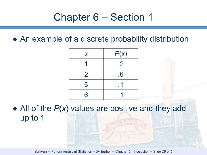
Chapter 6 – Section 1 ● An example of a discrete probability distribution x 1 2 5 P(x). 2. 6. 1 6 . 1 ● All of the P(x) values are positive and they add up to 1 Sullivan – Fundamentals of Statistics – 2 nd Edition – Chapter 5 Introduction – Slide 26 of 5
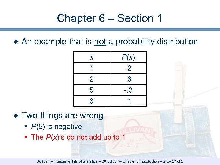
Chapter 6 – Section 1 ● An example that is not a probability distribution x 1 2 5 P(x). 2. 6 -. 3 6 . 1 ● Two things are wrong § P(5) is negative § The P(x)’s do not add up to 1 Sullivan – Fundamentals of Statistics – 2 nd Edition – Chapter 5 Introduction – Slide 27 of 5
Chapter 6 – Section 1 ● A probability histogram is a histogram where § The horizontal axis corresponds to the possible values of X (i. e. the x’s) § The vertical axis corresponds to the probabilities for those values (i. e. the P(x)’s) ● A probability histogram is very similar to a relative frequency histogram Sullivan – Fundamentals of Statistics – 2 nd Edition – Chapter 5 Introduction – Slide 28 of 5
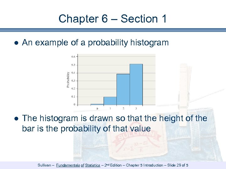
Chapter 6 – Section 1 ● An example of a probability histogram ● The histogram is drawn so that the height of the bar is the probability of that value Sullivan – Fundamentals of Statistics – 2 nd Edition – Chapter 5 Introduction – Slide 29 of 5
Chapter 6 – Section 1 ● The mean of a probability distribution can be thought of in this way: § There are various possible values of a discrete random variable § The values that have the higher probabilities are the ones that occur more often § The values that occur more often should have a larger role in calculating the mean § The mean is the weighted average of the values, weighted by the probabilities Sullivan – Fundamentals of Statistics – 2 nd Edition – Chapter 5 Introduction – Slide 30 of 5
Chapter 6 – Section 1 ● The mean of a discrete random variable is μX = Σ [ x • P(x) ] ● In this formula § x are the possible values of X § P(x) is the probability that x occurs § Σ means to add up these terms for all the possible values x Sullivan – Fundamentals of Statistics – 2 nd Edition – Chapter 5 Introduction – Slide 31 of 5
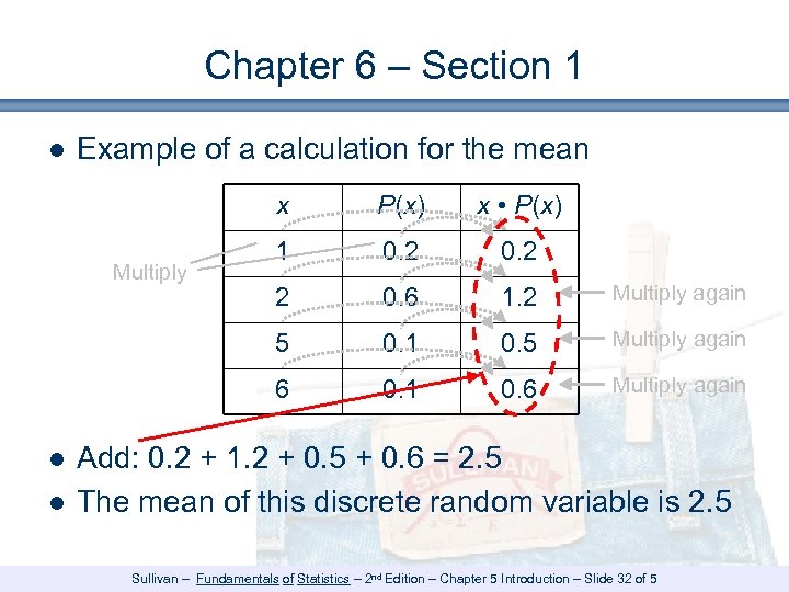
Chapter 6 – Section 1 ● Example of a calculation for the mean x x • P(x) 1 0. 2 2 0. 6 1. 2 Multiply again 5 0. 1 0. 5 Multiply again 6 Multiply P(x) 0. 1 0. 6 Multiply again ● Add: 0. 2 + 1. 2 + 0. 5 + 0. 6 = 2. 5 ● The mean of this discrete random variable is 2. 5 Sullivan – Fundamentals of Statistics – 2 nd Edition – Chapter 5 Introduction – Slide 32 of 5
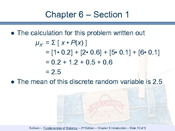
Chapter 6 – Section 1 ● The calculation for this problem written out μX = Σ [ x • P(x) ] = [1 • 0. 2] + [2 • 0. 6] + [5 • 0. 1] + [6 • 0. 1] = 0. 2 + 1. 2 + 0. 5 + 0. 6 = 2. 5 ● The mean of this discrete random variable is 2. 5 Sullivan – Fundamentals of Statistics – 2 nd Edition – Chapter 5 Introduction – Slide 33 of 5
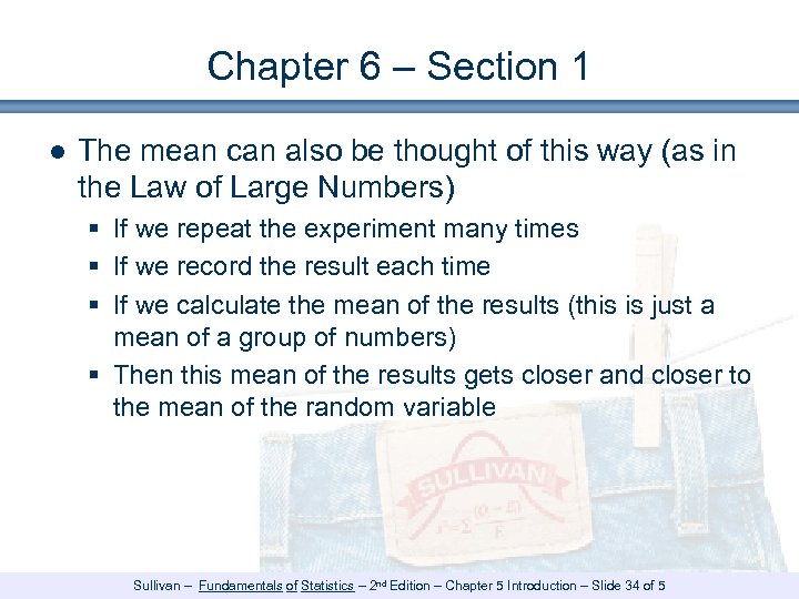
Chapter 6 – Section 1 ● The mean can also be thought of this way (as in the Law of Large Numbers) § If we repeat the experiment many times § If we record the result each time § If we calculate the mean of the results (this is just a mean of a group of numbers) § Then this mean of the results gets closer and closer to the mean of the random variable Sullivan – Fundamentals of Statistics – 2 nd Edition – Chapter 5 Introduction – Slide 34 of 5
Chapter 6 – Section 1 ● The expected value of a random variable is another term for its mean ● The term “expected value” illustrates the long term nature of the experiments – as we perform more and more experiments, the mean of the results of those experiments gets closer to the “expected value” of the random variable Sullivan – Fundamentals of Statistics – 2 nd Edition – Chapter 5 Introduction – Slide 35 of 5
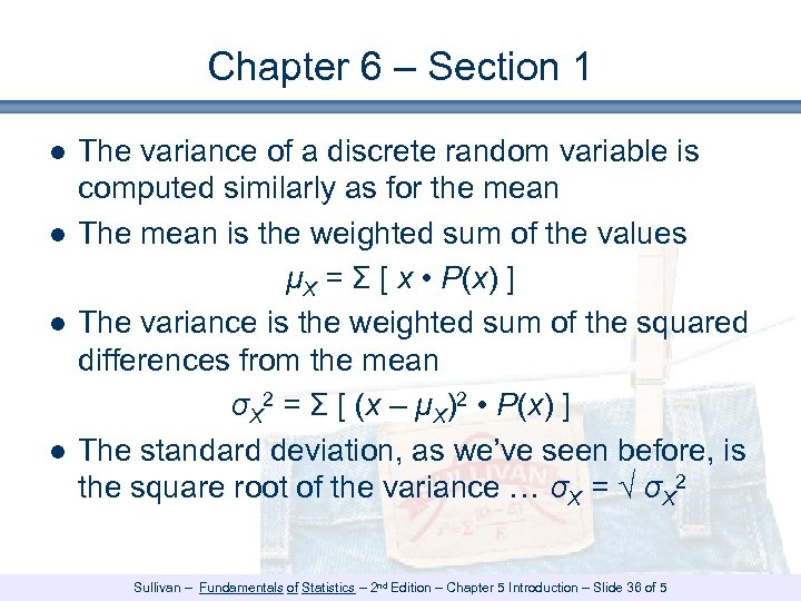
Chapter 6 – Section 1 ● The variance of a discrete random variable is computed similarly as for the mean ● The mean is the weighted sum of the values μX = Σ [ x • P(x) ] ● The variance is the weighted sum of the squared differences from the mean σX 2 = Σ [ (x – μX)2 • P(x) ] ● The standard deviation, as we’ve seen before, is the square root of the variance … σX = √ σX 2 Sullivan – Fundamentals of Statistics – 2 nd Edition – Chapter 5 Introduction – Slide 36 of 5
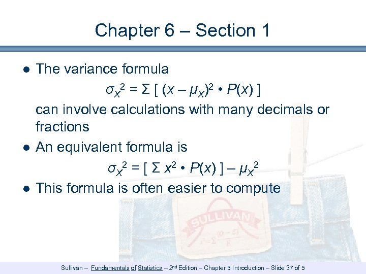
Chapter 6 – Section 1 ● The variance formula σX 2 = Σ [ (x – μX)2 • P(x) ] can involve calculations with many decimals or fractions ● An equivalent formula is σX 2 = [ Σ x 2 • P(x) ] – μX 2 ● This formula is often easier to compute Sullivan – Fundamentals of Statistics – 2 nd Edition – Chapter 5 Introduction – Slide 37 of 5
Chapter 6 – Section 1 ● For variables and samples (section 3. 2), we had the concept of a population variance (for the entire population) and a sample variance (for a sample from that population) ● These probability distributions model the complete population § These are population variance formulas § There is no analogy for sample variance here Sullivan – Fundamentals of Statistics – 2 nd Edition – Chapter 5 Introduction – Slide 38 of 5
Chapter 6 – Section 1 ● The variance can be calculated by hand, but the calculation is very tedious ● Whenever possible, use technology (calculators, software programs, etc. ) to calculate variances and standard deviations Sullivan – Fundamentals of Statistics – 2 nd Edition – Chapter 5 Introduction – Slide 39 of 5
Summary: Chapter 6 – Section 1 ● Discrete random variables are measures of outcomes that have discrete values ● Discrete random variables are specified by their Discrete probability distributions ● The mean of a discrete random variable can be interpreted as the long term average of repeated independent experiments ● The variance of a discrete random variable measures its dispersion from its mean Sullivan – Fundamentals of Statistics – 2 nd Edition – Chapter 5 Introduction – Slide 40 of 5
Chapter 6 Section 2 The Binomial Probability Distribution Sullivan – Fundamentals of Statistics – 2 nd Edition – Chapter 5 Introduction – Slide 41 of 5
Chapter 6 – Section 2 ● A binomial experiment has the following structure § The first test is performed … the result is either a success or a failure § The second test is performed … the result is either a success or a failure. This result is independent of the first and the chance of success is the same § A third test is performed … the result is either a success or a failure. The result is independent of the first two and the chance of success is the same Sullivan – Fundamentals of Statistics – 2 nd Edition – Chapter 5 Introduction – Slide 42 of 5
Chapter 6 – Section 2 ● Example § A card is drawn from a deck. A “success” is for that card to be a heart … a “failure” is for any other suit § The card is then put back into the deck § A second card is drawn from the deck with the same definition of success. § The second card is put back into the deck § We continue for 10 cards Sullivan – Fundamentals of Statistics – 2 nd Edition – Chapter 5 Introduction – Slide 43 of 5
Chapter 6 – Section 2 ● A binomial experiment is an experiment with the following characteristics § The experiment is performed a fixed number of times, each time called a trial § The trials are independent § Each trial has two possible outcomes, usually called a success and a failure § The probability of success is the same for every trial Sullivan – Fundamentals of Statistics – 2 nd Edition – Chapter 5 Introduction – Slide 44 of 5
Chapter 6 – Section 2 ● Notation used for binomial distributions § The number of trials is represented by n § The probability of a success is represented by p § The total number of successes in n trials is represented by X ● Because there cannot be a negative number of successes, and because there cannot be more than n successes (out of n attempts) 0≤X≤n Sullivan – Fundamentals of Statistics – 2 nd Edition – Chapter 5 Introduction – Slide 45 of 5
Chapter 6 – Section 2 ● In our card drawing example § Each trial is the experiment of drawing one card § The experiment is performed 10 times, so n = 10 § The trials are independent because the drawn card is put back into the deck § Each trial has two possible outcomes, a “success” of drawing a heart and a “failure” of drawing anything else § The probability of success is 0. 25, the same for every trial, so p = 0. 25 § X, the number of successes, is between 0 and 10 Sullivan – Fundamentals of Statistics – 2 nd Edition – Chapter 5 Introduction – Slide 46 of 5
Chapter 6 – Section 2 ● We would like to calculate the probabilities of X, i. e. P(0), P(1), P(2), …, P(n) ● Do a simpler example first § For n = 3 trials § With p =. 4 probability of success § Calculate P(2), the probability of 2 successes Sullivan – Fundamentals of Statistics – 2 nd Edition – Chapter 5 Introduction – Slide 47 of 5
Chapter 6 – Section 2 ● For 3 trials, the possible ways of getting exactly 2 successes are § S S F § S F S § F S S ● The probabilities for each (using the multiplication rule) are § 0. 4 • 0. 6 = 0. 096 § 0. 4 • 0. 6 • 0. 4 = 0. 096 § 0. 6 • 0. 4 = 0. 096 Sullivan – Fundamentals of Statistics – 2 nd Edition – Chapter 5 Introduction – Slide 48 of 5
Chapter 6 – Section 2 ● The total probability is P(2) = 0. 096 + 0. 096 = 0. 288 ● But there is a pattern § Each way had the same probability … the probability of 2 success (0. 4 times 0. 4) times the probability of 1 failure (0. 6 times 0. 6) ● The probability for each case is 0. 42 • 0. 61 Sullivan – Fundamentals of Statistics – 2 nd Edition – Chapter 5 Introduction – Slide 49 of 5
Chapter 6 – Section 2 ● There are 3 cases § S S F could represent choosing a combination of 2 out of 3 … choosing the first and the second § S F S could represent choosing a second combination of 2 out of 3 … choosing the first and the third § F S S could represent choosing a third combination of 2 out of 3 ● These are the 3 = 3 C 2 ways to choose 2 out of 3 Sullivan – Fundamentals of Statistics – 2 nd Edition – Chapter 5 Introduction – Slide 50 of 5
Chapter 6 – Section 2 ● Thus the total probability P(2) =. 096 +. 096 =. 288 can also be written as P(2) = 3 C 2 • . 42 • . 61 ● In other words, the probability is § The number of ways of choosing 2 out of 3, times § The probability of 2 successes, times § The probability of 1 failure Sullivan – Fundamentals of Statistics – 2 nd Edition – Chapter 5 Introduction – Slide 51 of 5
Chapter 6 – Section 2 ● The general formula for the binomial probabilities is just this ● For P(x), the probability of x successes, the probability is § The number of ways of choosing x out of n, times § The probability of x successes, times § The probability of n-x failures ● This formula is P(x) = n. Cx px (1 – p)n-x Sullivan – Fundamentals of Statistics – 2 nd Edition – Chapter 5 Introduction – Slide 52 of 5
Chapter 6 – Section 2 ● Example ● A student guesses at random on a multiple choice quiz § There are n = 10 questions in total § There are 5 choices per question so that the probability of success p = 1/5 =. 2 ● What is the probability that the student gets 6 questions correct? Sullivan – Fundamentals of Statistics – 2 nd Edition – Chapter 5 Introduction – Slide 53 of 5
Chapter 6 – Section 2 ● Example continued ● This is a binomial experiment § There a finite number n = 10 of trials § Each trial has two outcomes (a correct guess and an incorrect guess) § The probability of success is independent from trial to trial (every one is a random guess) § The probability of success p =. 2 is the same for each trial Sullivan – Fundamentals of Statistics – 2 nd Edition – Chapter 5 Introduction – Slide 54 of 5
Chapter 6 – Section 2 ● Example continued ● The probability of 6 correct guesses is P(x) = n. Cx px (1 – p)n-x = 6 C 10. 26. 84 = 210 • . 000064 • . 4096 =. 005505 ● This is less than a 1% chance ● In fact, the chance of getting 6 or more correct (i. e. a passing score) is also less than 1% Sullivan – Fundamentals of Statistics – 2 nd Edition – Chapter 5 Introduction – Slide 55 of 5
Chapter 6 – Section 2 ● Binomial calculations can be difficult because of the large numbers (the n. Cx) times the small numbers (the px and (1 -p)n-x) ● It is possible to use tables to look up these probabilities ● It is best to use a calculator routine or a software program to compute these probabilities Sullivan – Fundamentals of Statistics – 2 nd Edition – Chapter 5 Introduction – Slide 56 of 5
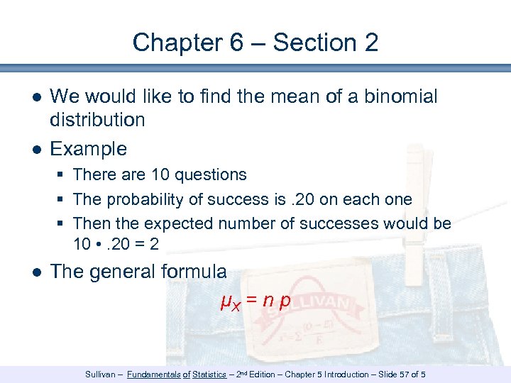
Chapter 6 – Section 2 ● We would like to find the mean of a binomial distribution ● Example § There are 10 questions § The probability of success is. 20 on each one § Then the expected number of successes would be 10 • . 20 = 2 ● The general formula μX = n p Sullivan – Fundamentals of Statistics – 2 nd Edition – Chapter 5 Introduction – Slide 57 of 5
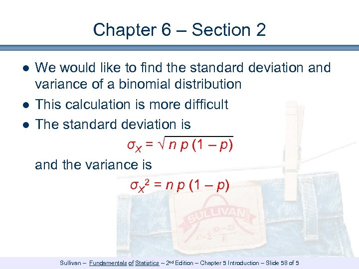
Chapter 6 – Section 2 ● We would like to find the standard deviation and variance of a binomial distribution ● This calculation is more difficult ● The standard deviation is σX = √ n p (1 – p) and the variance is σX 2 = n p (1 – p) Sullivan – Fundamentals of Statistics – 2 nd Edition – Chapter 5 Introduction – Slide 58 of 5
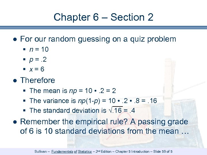
Chapter 6 – Section 2 ● For our random guessing on a quiz problem § n = 10 § p =. 2 § x=6 ● Therefore § The mean is np = 10 • . 2 = 2 § The variance is np(1 -p) = 10 • . 2 • . 8 =. 16 § The standard deviation is √. 16 =. 4 ● Remember the empirical rule? A passing grade of 6 is 10 standard deviations from the mean … Sullivan – Fundamentals of Statistics – 2 nd Edition – Chapter 5 Introduction – Slide 59 of 5
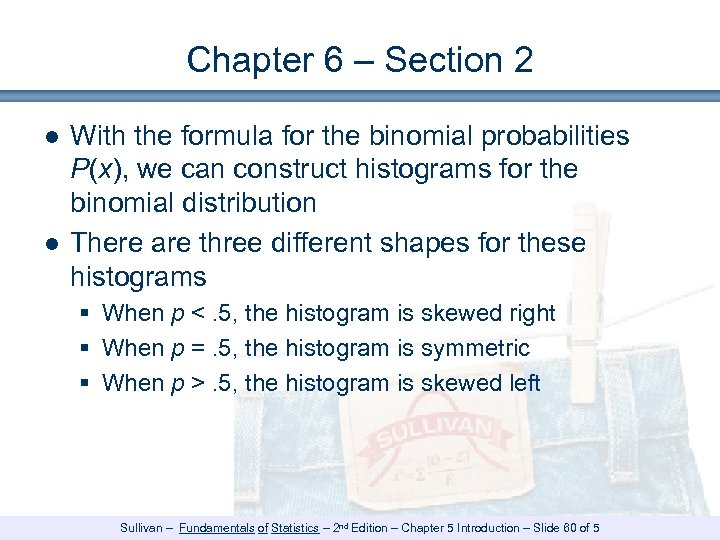
Chapter 6 – Section 2 ● With the formula for the binomial probabilities P(x), we can construct histograms for the binomial distribution ● There are three different shapes for these histograms § When p <. 5, the histogram is skewed right § When p =. 5, the histogram is symmetric § When p >. 5, the histogram is skewed left Sullivan – Fundamentals of Statistics – 2 nd Edition – Chapter 5 Introduction – Slide 60 of 5
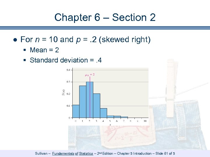
Chapter 6 – Section 2 ● For n = 10 and p =. 2 (skewed right) § Mean = 2 § Standard deviation =. 4 Sullivan – Fundamentals of Statistics – 2 nd Edition – Chapter 5 Introduction – Slide 61 of 5
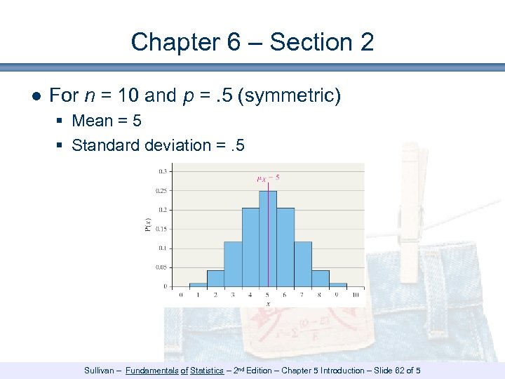
Chapter 6 – Section 2 ● For n = 10 and p =. 5 (symmetric) § Mean = 5 § Standard deviation =. 5 Sullivan – Fundamentals of Statistics – 2 nd Edition – Chapter 5 Introduction – Slide 62 of 5
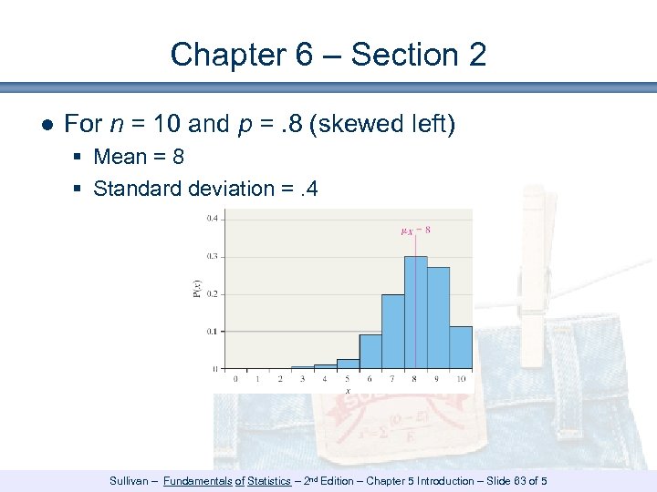
Chapter 6 – Section 2 ● For n = 10 and p =. 8 (skewed left) § Mean = 8 § Standard deviation =. 4 Sullivan – Fundamentals of Statistics – 2 nd Edition – Chapter 5 Introduction – Slide 63 of 5
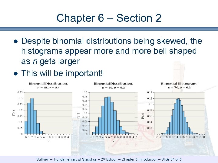
Chapter 6 – Section 2 ● Despite binomial distributions being skewed, the histograms appear more and more bell shaped as n gets larger ● This will be important! Sullivan – Fundamentals of Statistics – 2 nd Edition – Chapter 5 Introduction – Slide 64 of 5
Summary: Chapter 6 – Section 2 ● Binomial random variables model a series of independent trials, each of which can be a success or a failure, each of which has the same probability of success ● The binomial random variable has mean equal to np and variance equal to np(1 -p) Sullivan – Fundamentals of Statistics – 2 nd Edition – Chapter 5 Introduction – Slide 65 of 5
Chapter 6 Summary ● Discrete probability distributions § Random variables with discrete values § Models counts ● Binomial distribution § A sequence of success / failure trials § Models the number of successes Sullivan – Fundamentals of Statistics – 2 nd Edition – Chapter 5 Introduction – Slide 66 of 5
a4694c3a12366a0fbe36638cac8f5fcf.ppt