Part II Market power Chapter 3 Static imperfect

Part II. Market power Chapter 3. Static imperfect competition MATH SLIDES Slides Industrial Organization: Markets and Strategies Paul Belleflamme and Martin Peitz © Cambridge University Press 2009

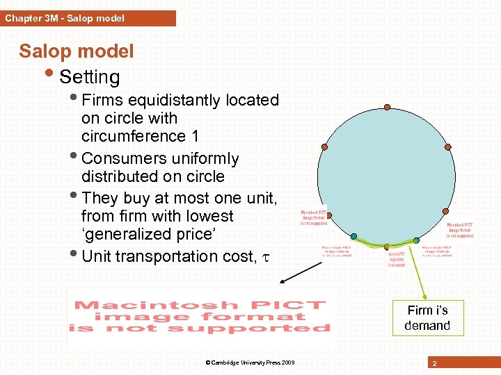Chapter 3 M - Salop model • Setting • Firms equidistantly located on circle with circumference 1 • Consumers uniformly distributed on circle • They buy at most one unit, from firm with lowest ‘generalized price’ • Unit transportation cost, Firm i’s demand © Cambridge University Press 2009 2

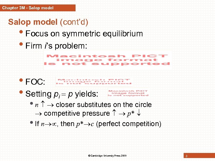Chapter 3 M - Salop model (cont’d) • Focus on symmetric equilibrium • Firm i’s problem: • FOC: • Setting pi p yields: • n closer substitutes on the circle competitive pressure p* • If n , then p* c (perfect competition) © Cambridge University Press 2009 3

Chapter 3 M - Asymmetric Hotelling Asymmetric competition with differentiated products • Same setting as Hotelling model • Only difference: product 1 is of superior quality difference • Consumer’s indirect utility: • Assume: r 2 r 1 product 2 more attractive for some consumers • Indifferent consumer © Cambridge University Press 2009 4

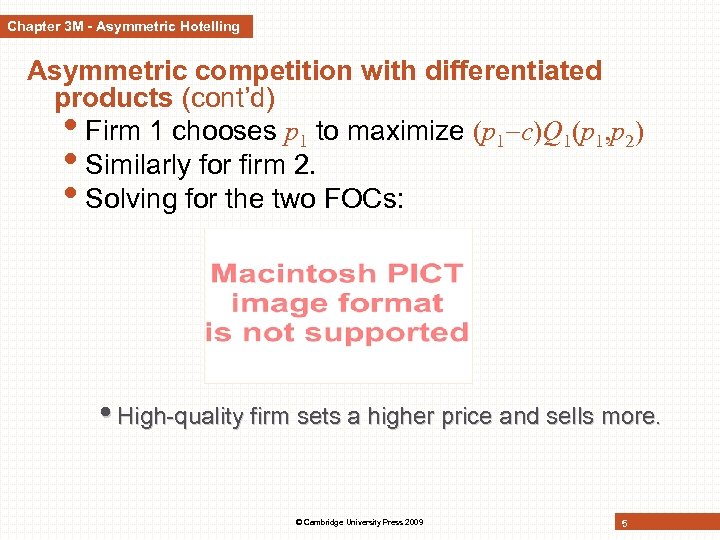Chapter 3 M - Asymmetric Hotelling Asymmetric competition with differentiated products (cont’d) • Firm 1 chooses p 1 to maximize (p 1 c)Q 1(p 1, p 2) • Similarly for firm 2. • Solving for the two FOCs: • High-quality firm sets a higher price and sells more. © Cambridge University Press 2009 5

Chapter 3 M - Asymmetric Hotelling Asymmetric competition with differentiated products (cont’d) • Welfare maximization sell at marginal cost • Firm 1’s equilibrium demand is too low from a social point of view. • Same analysis if r 1 r 2 r, but c 1 < c 2 • Lesson: Under imperfect competition, the firm with higher quality or lower marginal cost sells too few units from a welfare perspective. © Cambridge University Press 2009 6

Chapter 3 M - Asymmetric Hotelling Cournot pricing formula • F. O. C. of profit maximization for Cournot firm • Suppose constant marginal costs: Ci(qi) ciqi Lerner index (weighted by market shares) is proportional to Herfindahl index © Cambridge University Press 2009 7

Chapter 3 M - Kreps-Scheinkman Capacity-then-price model • Setting • Stage 1: firms set capacities 1 and incur cost of capacity, c • Stage 2: firms set prices pi; cost of production is up 2 to capacity (and infinite beyond capacity); demand is Q(p) a p. • Subgame-perfect equilibrium: firms know that capacity equilibrium choices may affect equilibrium prices • Efficient rationing • Upper bound on capacity at stage 1 © Cambridge University Press 2009 8

Chapter 3 M - Kreps-Scheinkman Capacity-then-price model (cont’d) • Claim: if c a (4/3)c, then both firms set the Claim market-clearing price: • Proof • Let p 1 p* and show that 2’s best-response is p 2 p*. • p 2 p* doesn’t pay: same quantity (because firm 2 sells all its capacity) sold at lower price • p 2 p* could pay as firm 1 is capacity constrained. . . For this, revenues should be increasing at p*. . . • Firm 2’s revenues: © Cambridge University Press 2009 9

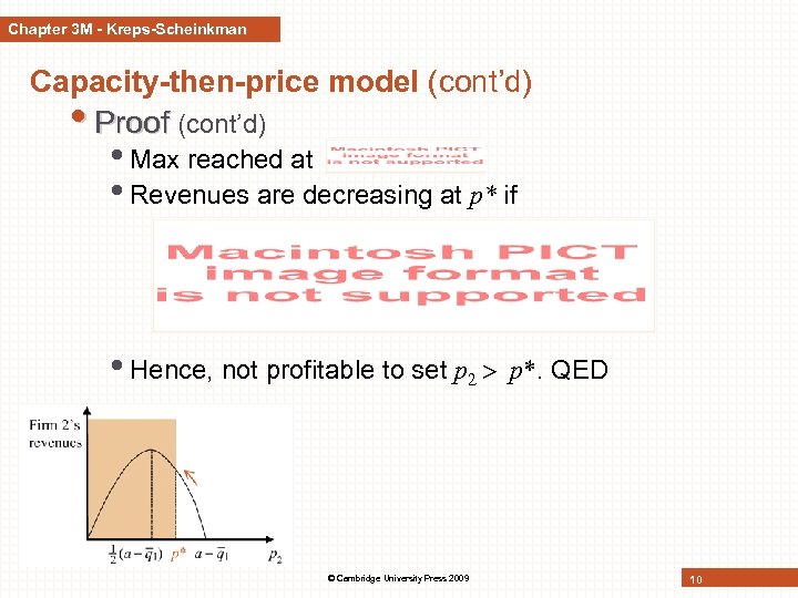Chapter 3 M - Kreps-Scheinkman Capacity-then-price model (cont’d) • Proof (cont’d) • Max reached at • Revenues are decreasing at p* if • Hence, not profitable to set p 2 p*. QED © Cambridge University Press 2009 10