6541558b9405134fa7c7f7efc5520206.ppt
- Количество слайдов: 51

Part 1 Introductory to Scilab Course
Outline Views 1. 0 Introduction to Scilab 2. 0 Scilab Environment 3. 0 Working with Variables and Array 4. 0 Scilab Programming Language 5. 0 Plotting and Visualization
Introduction - What is Scilab? ? • • • Scientific software package for numerical computations -> a powerful open computing environment for engineering and scientific applications An open source software Currently used in educational and industrial around the world Under Scilab Consortium – launched in May 2003 Includes hundreds of mathematical functions with the possibility to add interactively programs from various languages (C, C++, Fontran and etc) Has sophisticated data structures (including lists, polynomials, rational functions, linear systems & etc), an interpreter and a high level programming
Introduction - What is Scilab? ? Cntd. . What people like: • Can port a Matlab toolboxes to Scilab • Have impressive number of built-in functions as well as number of built-in toolboxes • Contain Scicos, a visual system modelling tool, letting the user visually build systems that can then be dynamically simulated. • Scicos is free counterpart to The Math. Work’s Simulink product, which must be purchased separately from Matlab. • Use without worrying about legality issues or (ethics!) It is FREEE!!! (erm. . . not interested BECAUSE we can get FREE pirated copy software!!!)
Introduction - What is Scilab? ? Cntd. . Primary issues/challenges: • Lack of a nice IDE (Integrated Development Environment). • It is not-really-free-licence. • The statement from the developers (from Scilab website) mention that the coming version 5 will be released under recognised open source licence.

What does it mean for Government, School or an Institution (GSI)? • Lower IT costs • Examples: Cost estimated to buy Matlab licence in Uni. MAP = 7 labs x 70 PCs x RM 4000 = RM 1, 960, 000. 00 • Spend more than a million just to install Matlab!! • Matlab is superb, but it may put you in the poor house! • If we don’t buy Matlab licence, the money can be used to buy other equipments which are more important for student usage.
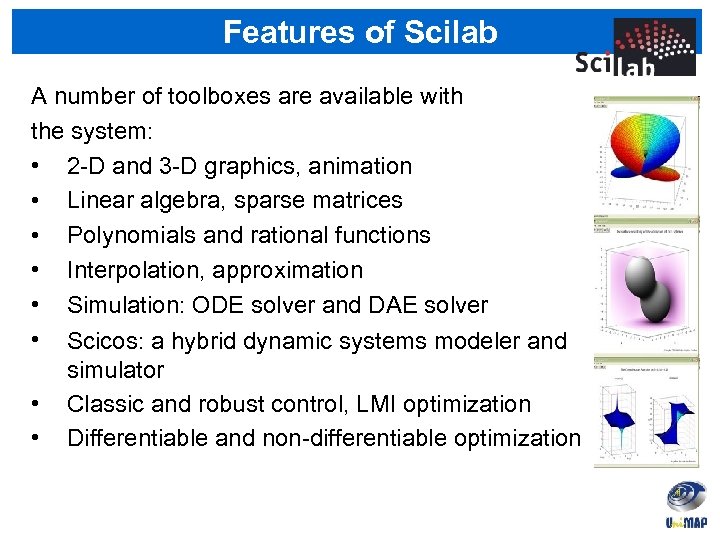
Features of Scilab A number of toolboxes are available with the system: • 2 -D and 3 -D graphics, animation • Linear algebra, sparse matrices • Polynomials and rational functions • Interpolation, approximation • Simulation: ODE solver and DAE solver • Scicos: a hybrid dynamic systems modeler and simulator • Classic and robust control, LMI optimization • Differentiable and non-differentiable optimization
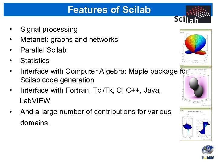
Features of Scilab • • Signal processing Metanet: graphs and networks Parallel Scilab Statistics Interface with Computer Algebra: Maple package for Scilab code generation Interface with Fortran, Tcl/Tk, C, C++, Java, Lab. VIEW And a large number of contributions for various domains.
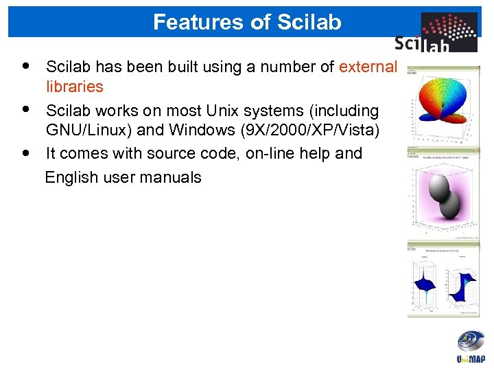
Features of Scilab • • • Scilab has been built using a number of external libraries Scilab works on most Unix systems (including GNU/Linux) and Windows (9 X/2000/XP/Vista) It comes with source code, on-line help and English user manuals

What’s next for Scilab in Uni. MAP? ? • Why use Scilab? Its capabilities to perform similar functions as Matlab such as: Design filter Plot graphs and spectrums Perform fast fourier transform (FFT) Perform signal analysis Simulate communication system design & etc • First implementation will be done for Signal and System lab module where Scilab with Linux platform will be used to replace Matlab software.

How to Install Scilab? • The simplest way to install and use Scilab is : Go to http: //www. scilab. org/ Download Scilab 5. 5. 2 (latest version) Run and follow its steps • To start Scilab : Double click the Scilab icon on the PC desktop or Go to Start / All Programs / Scilab / scilab (do not select Scilab Console)
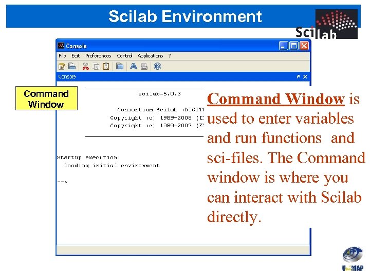
Scilab Environment Command Window is used to enter variables and run functions and sci-files. The Command window is where you can interact with Scilab directly.
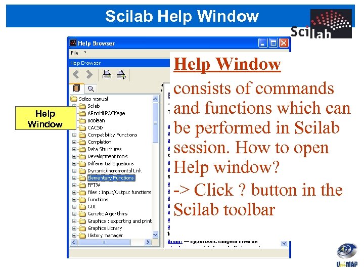
Scilab Help Window consists of commands and functions which can be performed in Scilab session. How to open Help window? -> Click ? button in the Scilab toolbar
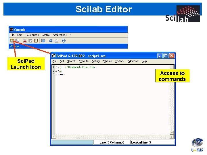
Scilab Editor Sci. Pad Launch Icon Access to commands
Workings with Variables and Array • • The Scilab environment is command oriented like UNIX. A prompt appears on the screen and a MATLAB statement can be entered. When the <ENTER> key is pressed, the statement is executed, and another prompt appears. If a statement is terminated with a semicolon ( ; ), no results will be displayed (similar to MATLAB). Variable names ARE case sensitive. Variable names must start with a letter followed by letters, digits, and underscores. Variable names and their types do not have to be declared. Any variable can take real, complex, and integer values. The name of variable is not accepted if it is reserved word.
Scilab Variables • Special variables: – ans: default variable name for the result. – %pi: π = 3. 1415926 => % is used in front of defined keyword - %i : i is an imaginary number - %inf : infinity (∞) • Commands involving variables: -who: lists the names of the defined variables -whos: lists entire contents of the workspace, including functions, libraries, constants -clear: clears all variables -clc: clears the command window clf: clears all plots in the active graphic window
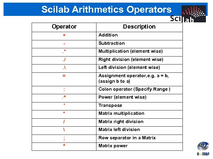
Scilab Arithmetics Operator Description + Addition - Subtraction . * Multiplication (element wise) . / Right division (element wise) . Left division (element wise) = Assignment operator, e. g. a = b, (assign b to a) : Colon operator (Specify Range ) . ^ Power (element wise) ' Transpose * Matrix multiplication / Matrix right division Matrix left division ; Row separator in a Matrix ^ Matrix power
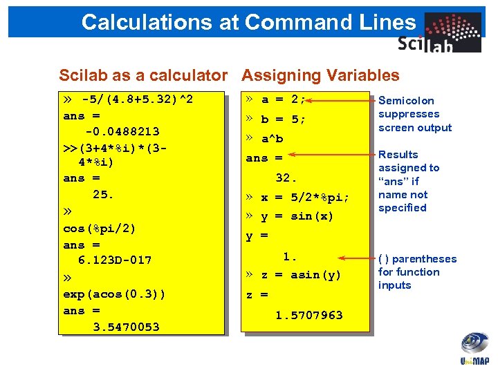
Calculations at Command Lines Scilab as a calculator Assigning Variables » a = 2; » -5/(4. 8+5. 32)^2 Semicolon ans = -0. 0488213 >>(3+4*%i)*(34*%i) ans = 25. » cos(%pi/2) ans = 6. 123 D-017 » exp(acos(0. 3)) ans = 3. 5470053 » b = 5; » a^b suppresses screen output ans = Results assigned to “ans” if name not specified 32. » x = 5/2*%pi; » y = sin(x) y = 1. » z = asin(y) z = 1. 5707963 ( ) parentheses for function inputs
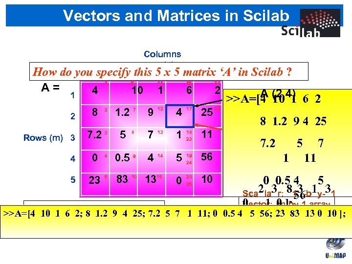
Vectors and Matrices in Scilab Columns (n) specify 2 this 5 x 5 matrix 1 3 4 How do you A= 4 1 6 10 1 2 Rows (m) 3 4 8 11 1 1. 2 7 9 12 7. 2 3 5 8 7 0 0. 5 9 4 2 4 16 ‘A’ 5 Scilab ? in 21 6 2 4 17 25 22 13 1 18 23 11 14 5 19 24 56 >>A=[A (2, 4) 6 2 4 10 1 8 1. 2 9 4 25 A (17) 7. 2 5 7 1 11 0 0. 5 Matrix: 5 Rectangular 4 Sca 2 la 3 r: 813 -b 1 y-31 56 0 arra 1 m-by-1 array Vector: y 0 ]; Matrix elements can be EITHER >>A=[4 10 1 6 2; 8 1. 2 9 4 25; 7. 2 5 7 1 11; 0 0. 5 4 5 56; 23 83 13 0 10 ]; 1 -by-n array numbers OR characters Matrix: m-by-n array 5 23 5 83 10 1315 0 20 25 10
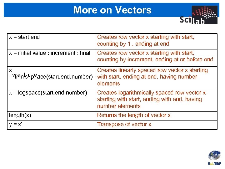
More on Vectors x = start: end Creates row vector x starting with start, counting by 1 , ending at end x = initial value : increment : final Creates row vector x starting with start, counting by increment, ending at or before end x Creates linearly spaced row vector x starting =vlianlsupeace(start, end, number) with start, ending at end, having number elements x = logspace(start, end, number) Creates logarithmically spaced row vector x starting with start, ending with end, having number elements length(x) Returns the length of vector x y = x’ Transpose of vector x
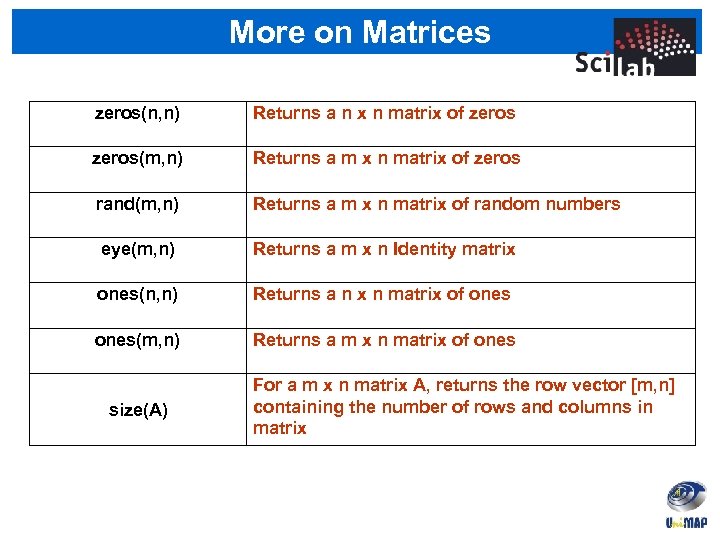
More on Matrices zeros(n, n) Returns a n x n matrix of zeros(m, n) Returns a m x n matrix of zeros rand(m, n) Returns a m x n matrix of random numbers eye(m, n) Returns a m x n Identity matrix ones(n, n) Returns a n x n matrix of ones(m, n) Returns a m x n matrix of ones size(A) For a m x n matrix A, returns the row vector [m, n] containing the number of rows and columns in matrix
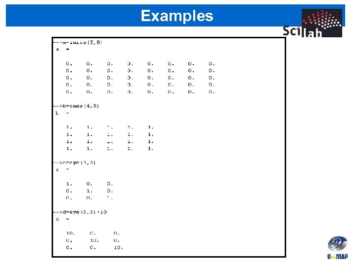
Examples
![Entering numeric array Use [ ] to combine existing arrays as matrix “elements” » Entering numeric array Use [ ] to combine existing arrays as matrix “elements” »](https://present5.com/presentation/6541558b9405134fa7c7f7efc5520206/image-23.jpg)
Entering numeric array Use [ ] to combine existing arrays as matrix “elements” » a=[1 2; 3 4] a = Column separator: space / comma (, ) The resulting matrix must be rectangular. 2 3 Row separator: semicolon (; ) 1 Use square brackets [ ] 4 » cat_a=[a, 2*a; 3*a, 4*a; 5*a, 6*a] cat_a = 1. 2. 2. . 4 3. 4. 6. 8. 3. 6. 4. 8. 4*a 9. 12. 16. 5. 10. 6. 12. 15. 20. 18. 24.
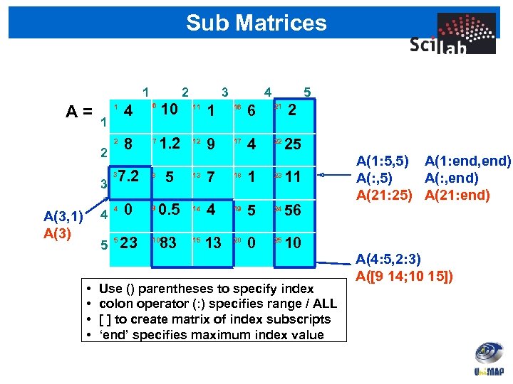
Sub Matrices 1 2 1 4 2 A= 8 7 1 2 7. 2 3 3 5 1 16 6 21 2 12 9 17 4 22 25 8 5 13 7 18 1 23 11 0. 5 14 4 19 5 24 56 83 15 13 20 0 25 10 4 0 9 5 • • 4 11 4 A(3, 1) A(3) 3 10 6 5 23 10 Use () parentheses to specify index colon operator (: ) specifies range / ALL [ ] to create matrix of index subscripts ‘end’ specifies maximum index value A(1: 5, 5) A(1: end, end) A(: , 5) A(: , end) A(21: 25) A(21: end) A(4: 5, 2: 3) A([9 14; 10 15])
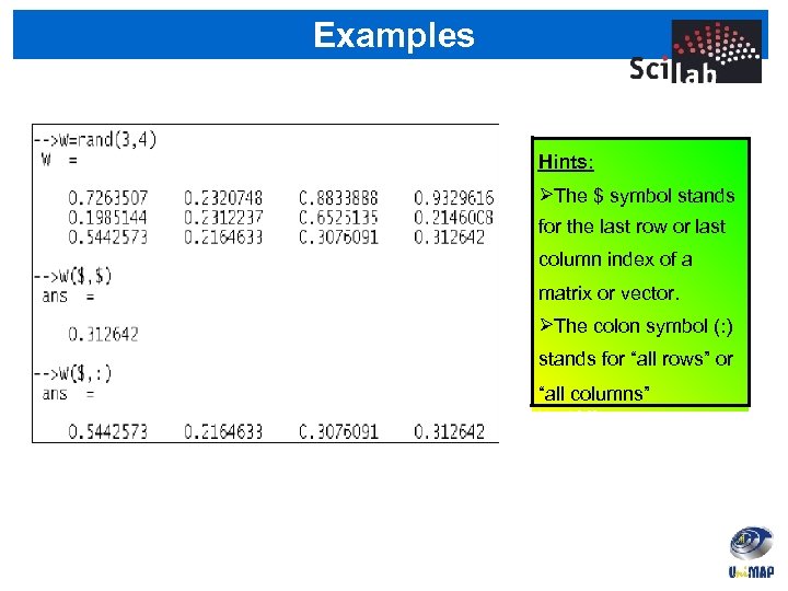
Examples Hints: The $ symbol stands for the last row or last column index of a matrix or vector. The colon symbol (: ) stands for “all rows” or “all columns”
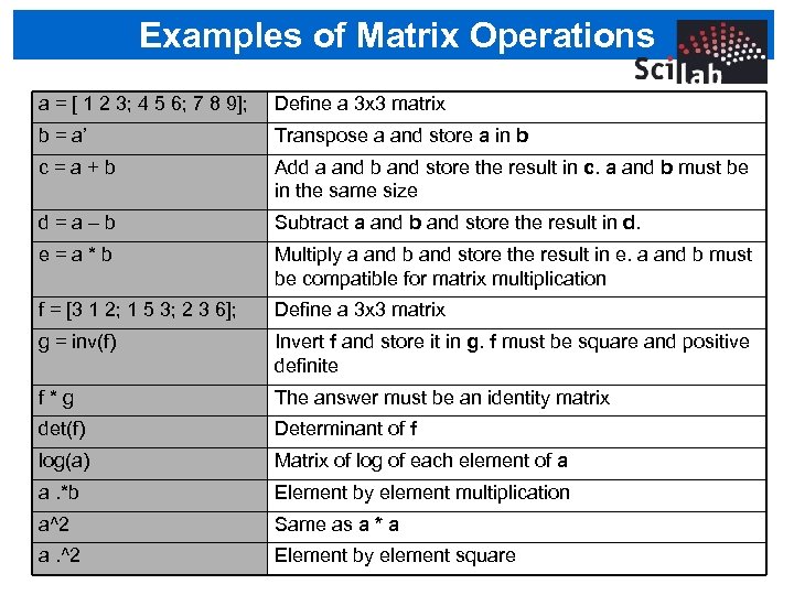
Examples of Matrix Operations a = [ 1 2 3; 4 5 6; 7 8 9]; Define a 3 x 3 matrix b = a’ Transpose a and store a in b c=a+b Add a and b and store the result in c. a and b must be in the same size d=a–b Subtract a and b and store the result in d. e=a*b Multiply a and b and store the result in e. a and b must be compatible for matrix multiplication f = [3 1 2; 1 5 3; 2 3 6]; Define a 3 x 3 matrix g = inv(f) Invert f and store it in g. f must be square and positive definite f*g The answer must be an identity matrix det(f) Determinant of f log(a) Matrix of log of each element of a a. *b Element by element multiplication a^2 Same as a * a a. ^2 Element by element square
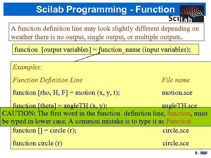
Scilab Programming - Function A function definition line may look slightly different depending on The syntax is a output, definition line is as follows…… weatherefor nofunction single output, or multiple outputs. function [output variables] = function_name (input variables); The function_name must be the same as the Examples: filename (without the. sce extension) in which the function is File name Function Definition Line written. For example if the name of the function is euler then it must F] written (x, t); with the function [rho, H, be = motion and y, saved in a file motion. sce name euler. sce function [theta] = angle. TH (x, y); angle. TH. sce CAUTION: The first word in the function definition line, function, must function theta = THETA (x, y, mistake is to type it as Function THETA. sce be typed in lower case. A common z); function [] = circle (r); circle. sce function circle (r) circle. sce
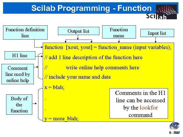
Scilab Programming - Function definition line Output list Function name Input list function [xout, yout] = function_name (input variables); H 1 line Comment line used by online help // add 1 line description of the function here // write online help comments here // include your name and date x = blah; Body of the function . . y = more_blah; Comments in the H 1 line can be accessed by the lookfor command
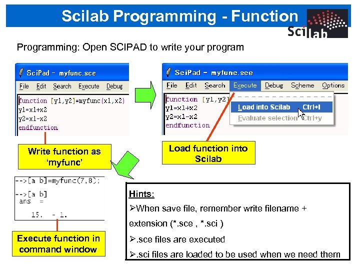
Scilab Programming - Function Programming: Open SCIPAD to write your program Load function into Scilab Write function as ‘myfunc’ Hints: When save file, remember write filename + extension (*. sce , *. sci ) Execute function in command window . sce files are executed . sci files are loaded to be used when we need them
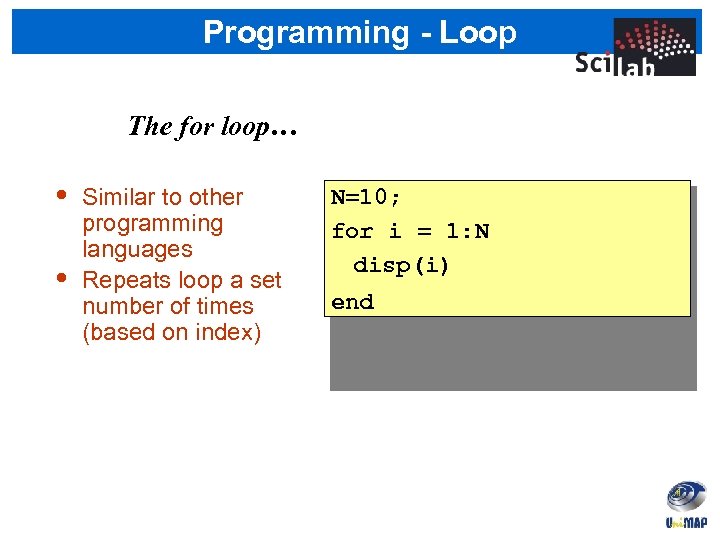
Programming - Loop The for loop… • • Similar to other programming languages Repeats loop a set number of times (based on index) N=10; for i = 1: N disp(i) end
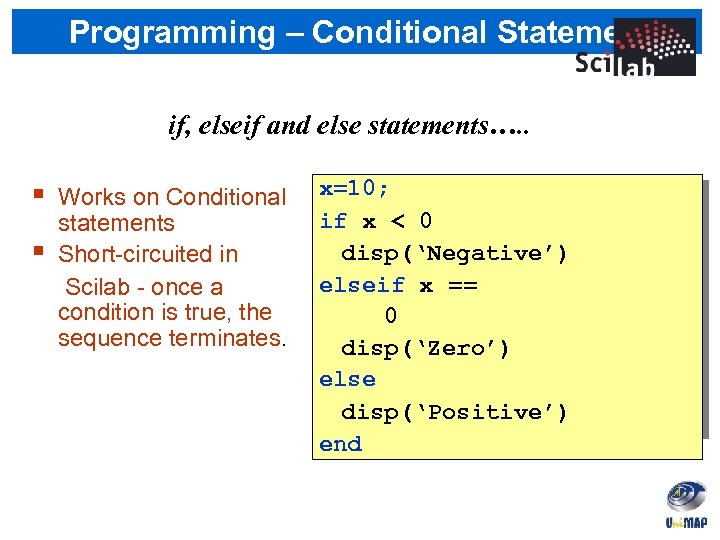
Programming – Conditional Statement if, elseif and else statements…. . Works on Conditional statements Short-circuited in Scilab - once a condition is true, the sequence terminates. x=10; if x < 0 disp(‘Negative’) elseif x == 0 disp(‘Zero’) else disp(‘Positive’) end
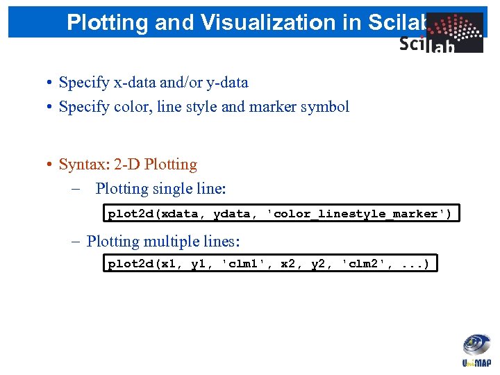
Plotting and Visualization in Scilab • Specify x-data and/or y-data • Specify color, line style and marker symbol • Syntax: 2 -D Plotting – Plotting single line: plot 2 d(xdata, ydata, 'color_linestyle_marker') – Plotting multiple lines: plot 2 d(x 1, y 1, 'clm 1', x 2, y 2, 'clm 2', . . . )
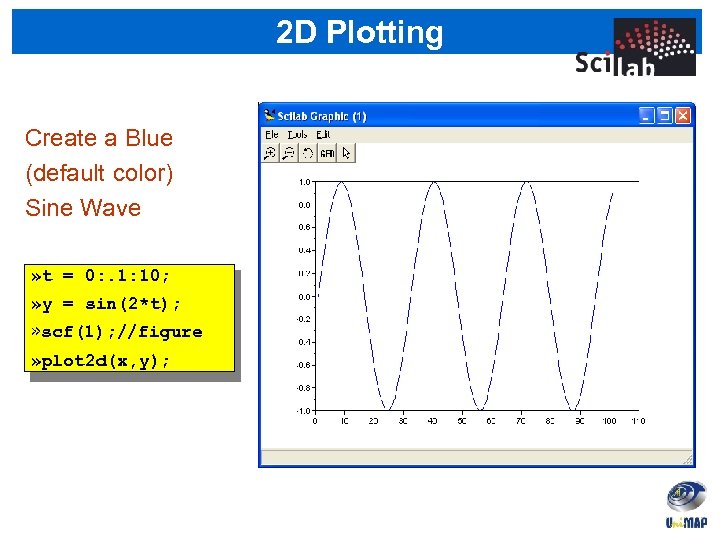
2 D Plotting Create a Blue (default color) Sine Wave » t = 0: . 1: 10; » y = sin(2*t); » scf(1); //figure » plot 2 d(x, y);
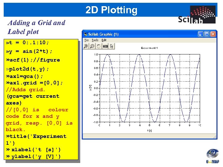
2 D Plotting Adding a Grid and Label plot » t = 0: . 1: 10; » y = sin(2*t); » scf(1); //figure » plot 2 d(t, y); » ax 1=gca(); » ax 1. grid =[0, 0]; //Adds grid. (gca=get current axes) //[0, 0] is colour code for x and y grid, resp. [0, 0] is black. » title('Experiment 1') » xlabel('t [s]') » ylabel('y [V]')
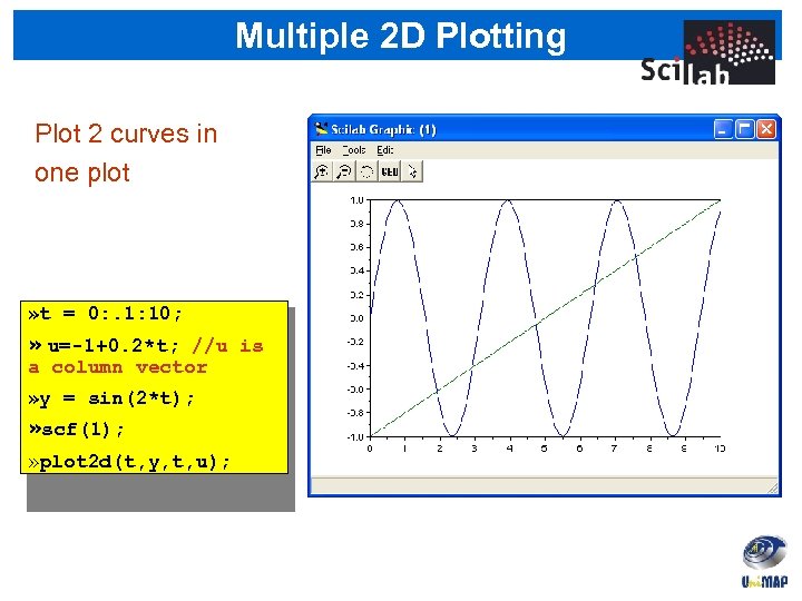
Multiple 2 D Plotting Plot 2 curves in one plot » t = 0: . 1: 10; » u=-1+0. 2*t; //u is a column vector » y = sin(2*t); » scf(1); » plot 2 d(t, y, t, u);
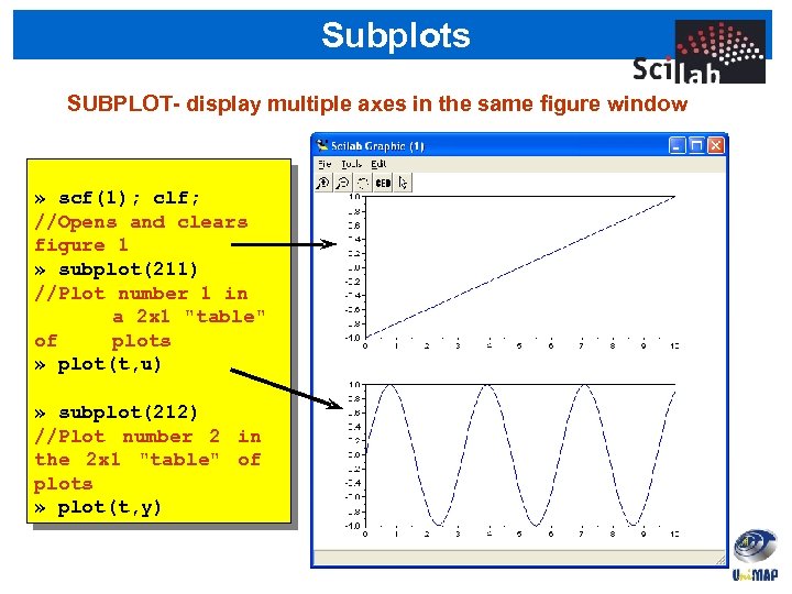
Subplots SUBPLOT- display multiple axes in the same figure window » scf(1); clf; //Opens and clears figure 1 » subplot(211) //Plot number 1 in a 2 x 1 "table" of plots » plot(t, u) » subplot(212) //Plot number 2 in the 2 x 1 "table" of plots » plot(t, y)
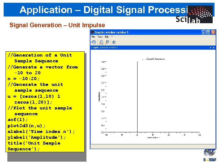
Application – Digital Signal Processing Signal Generation – Unit Impulse //Generation of a Unit Sample Sequence //Generate a vector from -10 to 20 n = -10: 20; //Generate the unit sample sequence u = [zeros(1, 10) 1 zeros(1, 20)]; //Plot the unit sample sequence scf(1); plot 2 d 3(n, u); xlabel('Time index n'); ylabel('Amplitude'); title('Unit Sample Sequence');
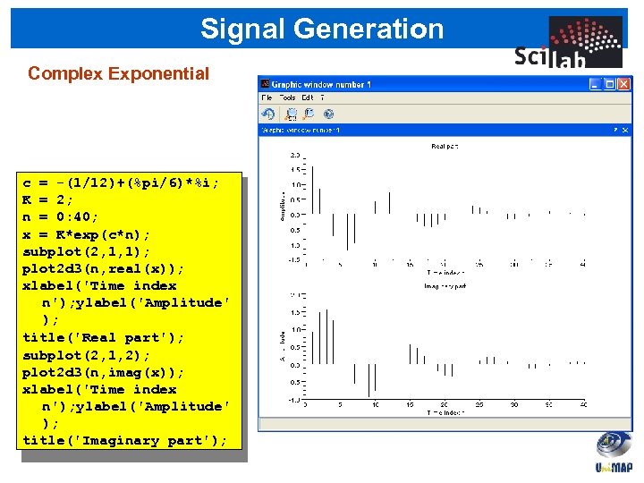
Signal Generation Complex Exponential c = -(1/12)+(%pi/6)*%i; K = 2; n = 0: 40; x = K*exp(c*n); subplot(2, 1, 1); plot 2 d 3(n, real(x)); xlabel('Time index n'); ylabel('Amplitude' ); title('Real part'); subplot(2, 1, 2); plot 2 d 3(n, imag(x)); xlabel('Time index n'); ylabel('Amplitude' ); title('Imaginary part');
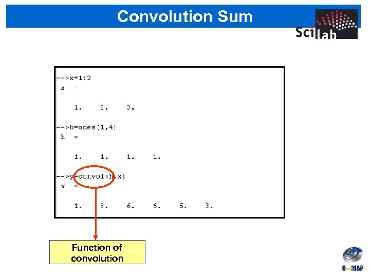
Convolution Sum Function of convolution
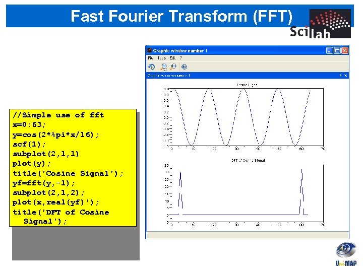
Fast Fourier Transform (FFT) //Simple use of fft x=0: 63; y=cos(2*%pi*x/16); scf(1); subplot(2, 1, 1) plot(y); title('Cosine Signal'); yf=fft(y, -1); subplot(2, 1, 2); plot(x, real(yf)'); title('DFT of Cosine Signal');
![Frequency Response in Z-Transform • Example: Given the difference equation as the following: y[n] Frequency Response in Z-Transform • Example: Given the difference equation as the following: y[n]](https://present5.com/presentation/6541558b9405134fa7c7f7efc5520206/image-41.jpg)
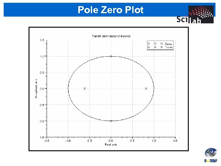
Frequency Response in Z-Transform • Example: Given the difference equation as the following: y[n] 0. 2 y[n 1] 0. 5 y[n 2] 2] x[n (i) Find zeroes and poles for the given H(z) and plot them (ii) Plot the magnitude and phase response of H(z)
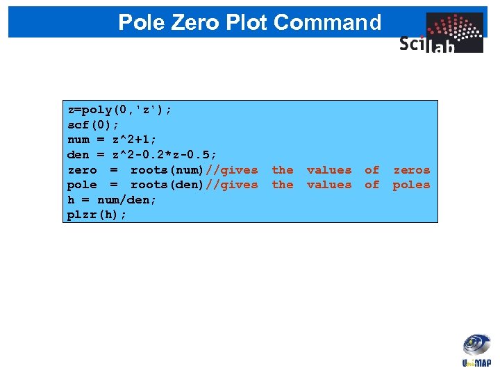
Pole Zero Plot Command z=poly(0, 'z'); scf(0); num = z^2+1; den = z^2 -0. 2*z-0. 5; zero = roots(num)//gives pole = roots(den)//gives h = num/den; plzr(h); the values of of zeros poles
Pole Zero Plot
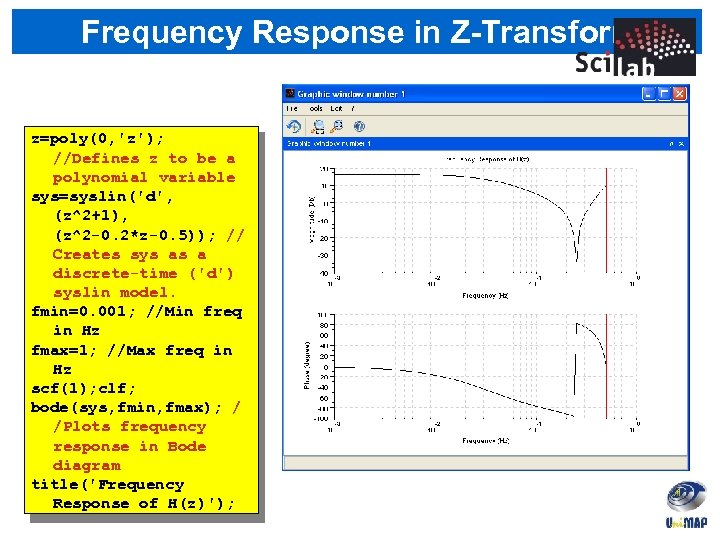
Frequency Response in Z-Transform z=poly(0, 'z'); //Defines z to be a polynomial variable sys=syslin('d', (z^2+1), (z^2 -0. 2*z-0. 5)); // Creates sys as a discrete-time ('d') syslin model. fmin=0. 001; //Min freq in Hz fmax=1; //Max freq in Hz scf(1); clf; bode(sys, fmin, fmax); / /Plots frequency response in Bode diagram title('Frequency Response of H(z)');
Frequency Response in Z-Transform • bode( ) plots frequency response in a Bode plot • The frequency axis shows normalized frequencies. • The red vertical line in the Bode plots represents the • normalized Nyquist frequency, which is 0. 5, corresponding to the normalized sampling frequency being 1 samples/sec. If the actual sampling frequency is fs [samples/sec], the actual (non-normalized) frequency is found by multiplying the normalized frequency by fs.
FIR Filter Design • To fully design and implement a filter, five steps are required: (1) Filter specification (2) Coefficient calculation (3) Structure selection (4) Simulation (optional) - MATLAB (5) Hardware Implementation (using FPGA or DSP board)
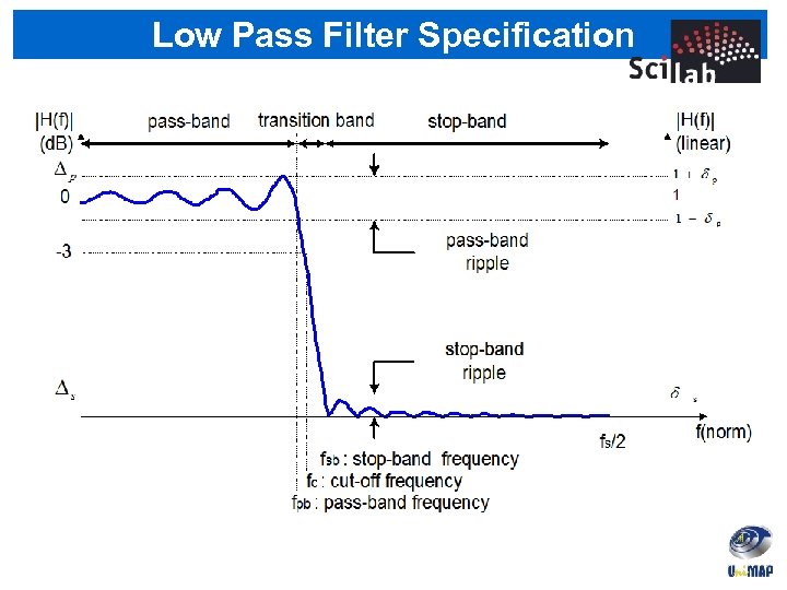
Low Pass Filter Specification
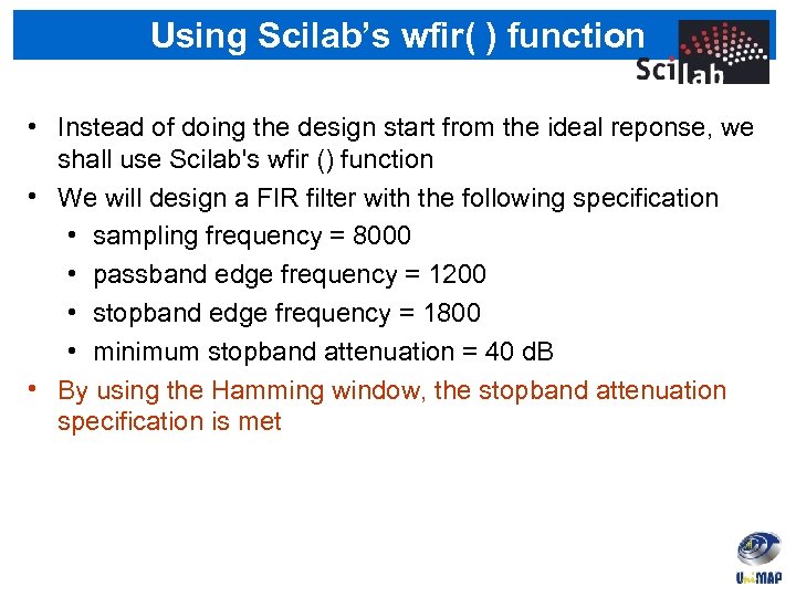
Using Scilab’s wfir( ) function • Instead of doing the design start from the ideal reponse, we shall use Scilab's wfir () function • We will design a FIR filter with the following specification • sampling frequency = 8000 • passband edge frequency = 1200 • stopband edge frequency = 1800 • minimum stopband attenuation = 40 d. B • By using the Hamming window, the stopband attenuation specification is met
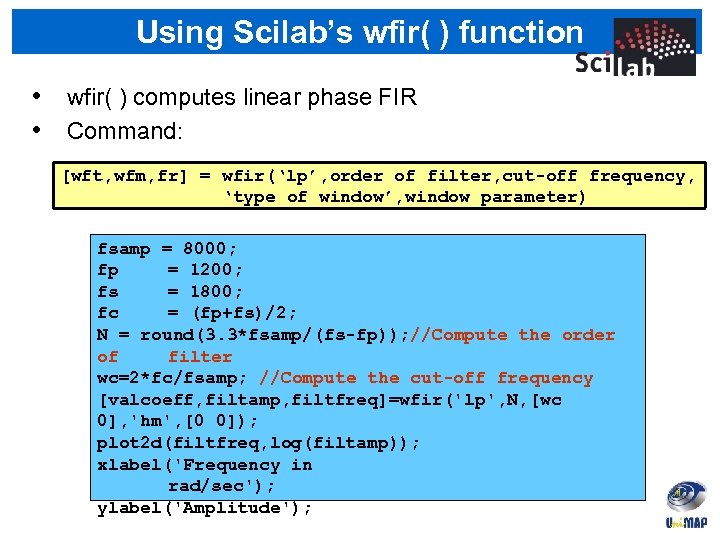
Using Scilab’s wfir( ) function • wfir( ) computes linear phase FIR • Command: [wft, wfm, fr] = wfir(‘lp’, order of filter, cut-off frequency, ‘type of window’, window parameter) fsamp = 8000; fp = 1200; fs = 1800; fc = (fp+fs)/2; N = round(3. 3*fsamp/(fs-fp)); //Compute the order of filter wc=2*fc/fsamp; //Compute the cut-off frequency [valcoeff, filtamp, filtfreq]=wfir('lp', N, [wc 0], 'hm', [0 0]); plot 2 d(filtfreq, log(filtamp)); xlabel('Frequency in rad/sec'); ylabel('Amplitude');
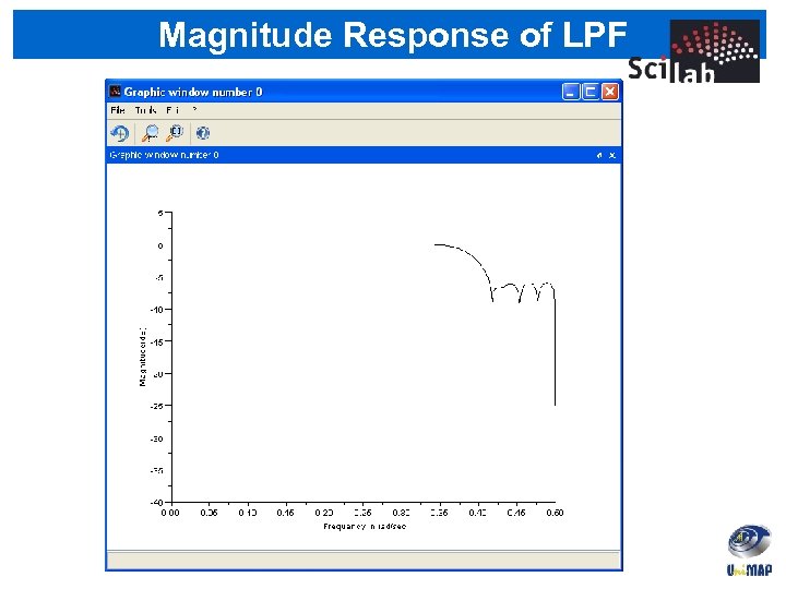
Magnitude Response of LPF

6541558b9405134fa7c7f7efc5520206.ppt