Parallel ICA Algorithm and Modeling Hongtao Du March

Parallel ICA Algorithm and Modeling Hongtao Du March 25, 2004

Outline l Review – – – l l l Independent Component Analysis Fast. ICA Parallel Computing Laws Parallel Computing Models Model for p. ICA

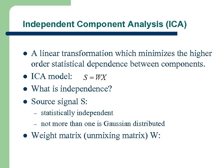Independent Component Analysis (ICA) l l A linear transformation which minimizes the higher order statistical dependence between components. ICA model: What is independence? Source signal S: – – l statistically independent not more than one is Gaussian distributed Weight matrix (unmixing matrix) W:

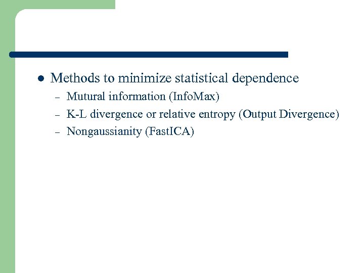l Methods to minimize statistical dependence – – – Mutural information (Info. Max) K-L divergence or relative entropy (Output Divergence) Nongaussianity (Fast. ICA)

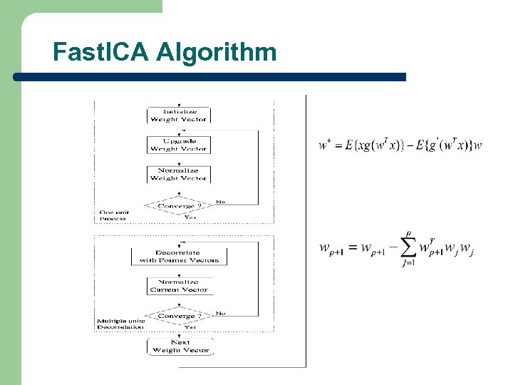Fast. ICA Algorithm

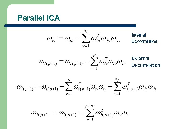Parallel ICA Internal Decorrelation External Decorrelation

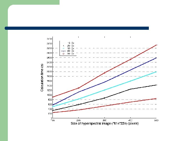
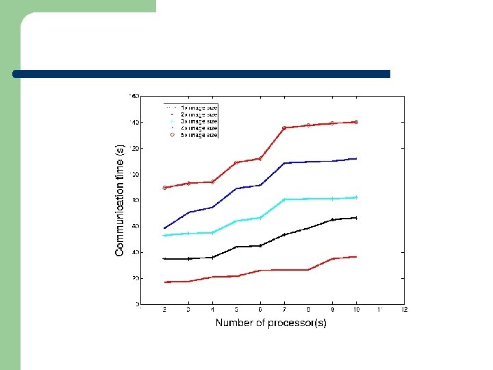
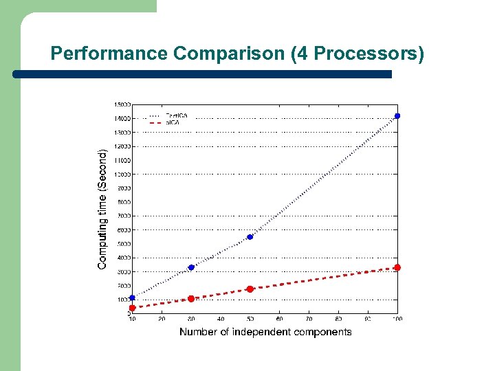Performance Comparison (4 Processors)

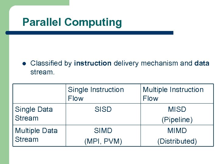Parallel Computing l Classified by instruction delivery mechanism and data stream. Single Instruction Flow Single Data Stream Multiple Data Stream SISD SIMD (MPI, PVM) Multiple Instruction Flow MISD (Pipeline) MIMD (Distributed)

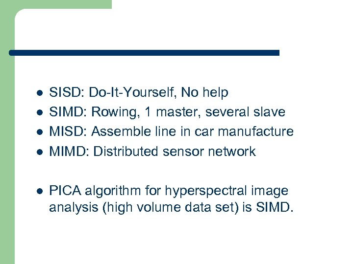l l l SISD: Do-It-Yourself, No help SIMD: Rowing, 1 master, several slave MISD: Assemble line in car manufacture MIMD: Distributed sensor network PICA algorithm for hyperspectral image analysis (high volume data set) is SIMD.

Parallel Computing Laws and Models l l Amdahl Law Gustafson Law BSP Model Log. P Model

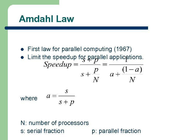Amdahl Law l l First law for parallel computing (1967) Limit the speedup for parallel applications. where N: number of processors s: serial fraction p: parallel fraction

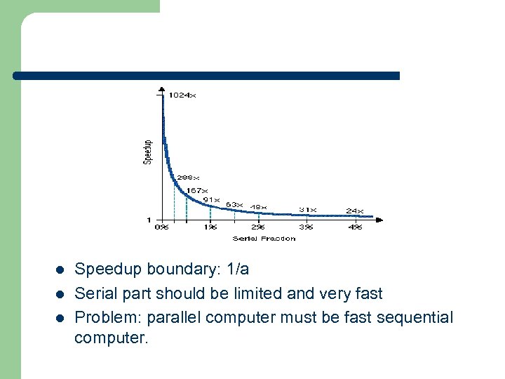l l l Speedup boundary: 1/a Serial part should be limited and very fast Problem: parallel computer must be fast sequential computer.

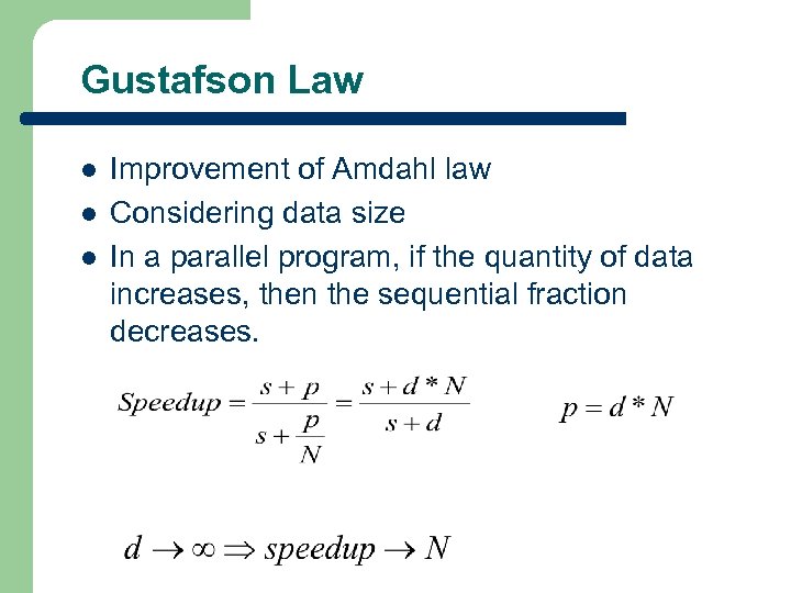Gustafson Law l l l Improvement of Amdahl law Considering data size In a parallel program, if the quantity of data increases, then the sequential fraction decreases.

Parallel Computing Model l Amdahl and Gustafson laws define the limits without considering the properties of the computer architecture Can not predict the real performance of any parallel application. Parallel computing models integrate the computer architecture and application architecture.

l Purpose: – – l Predicting computing cost Evaluating efficiency of programs Impacts on performance – – – Computing node (processor, memory) Communication network Tapp=Tcomp+Tcomm

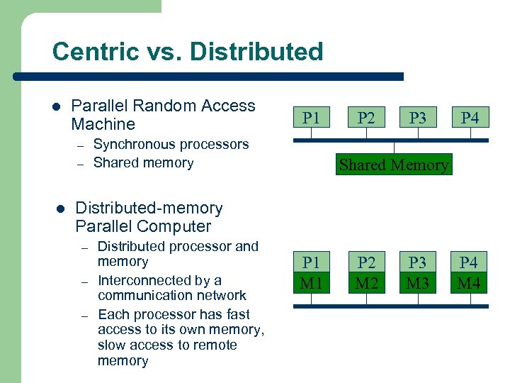Centric vs. Distributed l Parallel Random Access Machine – – l P 1 Synchronous processors Shared memory P 2 P 3 P 4 Shared Memory Distributed-memory Parallel Computer – – – Distributed processor and memory Interconnected by a communication network Each processor has fast access to its own memory, slow access to remote memory P 1 M 1 P 2 M 2 P 3 M 3 P 4 M 4

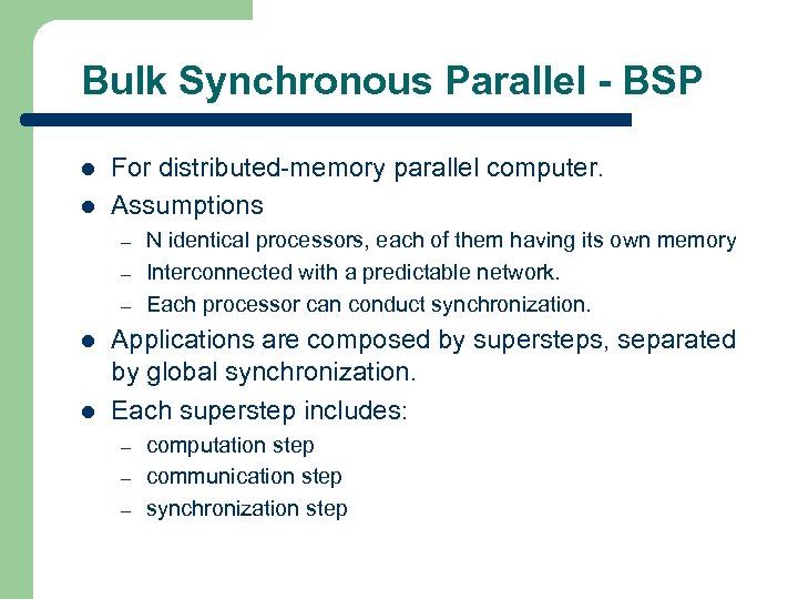Bulk Synchronous Parallel - BSP l l For distributed-memory parallel computer. Assumptions – – – l l N identical processors, each of them having its own memory Interconnected with a predictable network. Each processor can conduct synchronization. Applications are composed by supersteps, separated by global synchronization. Each superstep includes: – – – computation step communication step synchronization step

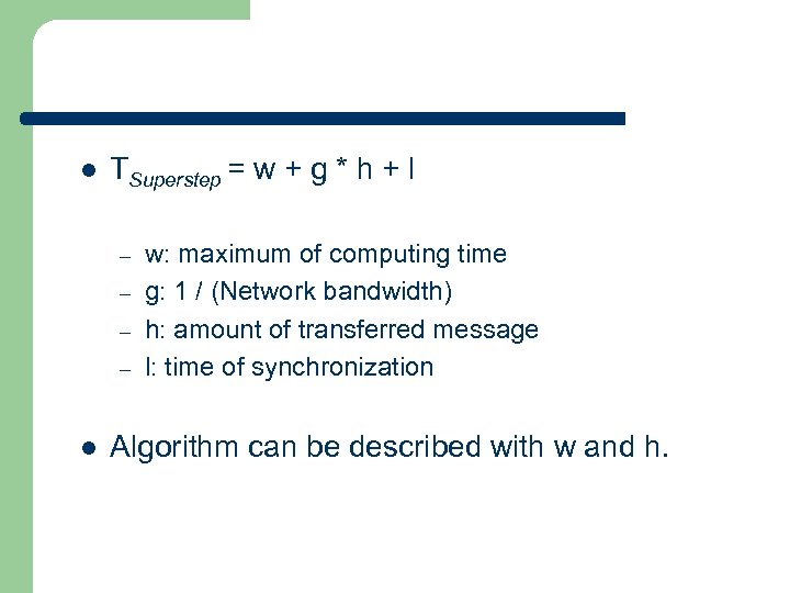l TSuperstep = w + g * h + l – – l w: maximum of computing time g: 1 / (Network bandwidth) h: amount of transferred message l: time of synchronization Algorithm can be described with w and h.

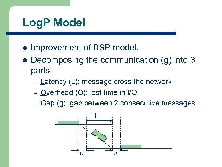Log. P Model l l Improvement of BSP model. Decomposing the communication (g) into 3 parts. – – – Latency (L): message cross the network Overhead (O): lost time in I/O Gap (g): gap between 2 consecutive messages L o o

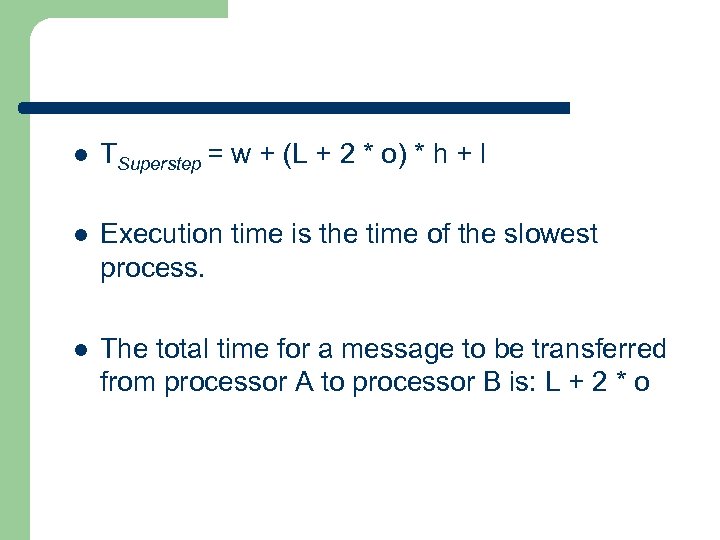l TSuperstep = w + (L + 2 * o) * h + l l Execution time is the time of the slowest process. l The total time for a message to be transferred from processor A to processor B is: L + 2 * o

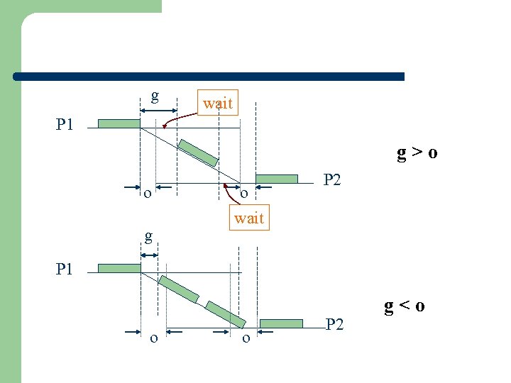g wait P 1 g>o o g o wait P 2 P 1 o o P 2 g

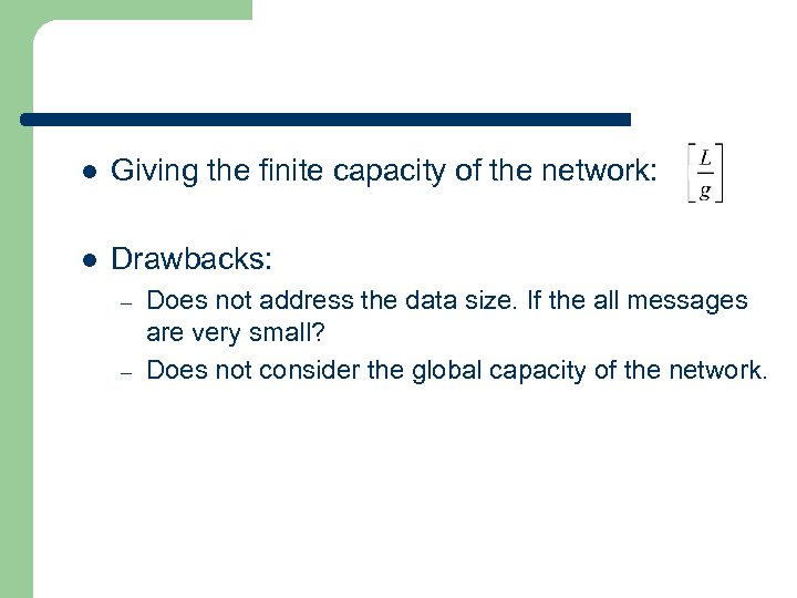l Giving the finite capacity of the network: l Drawbacks: – – Does not address the data size. If the all messages are very small? Does not consider the global capacity of the network.

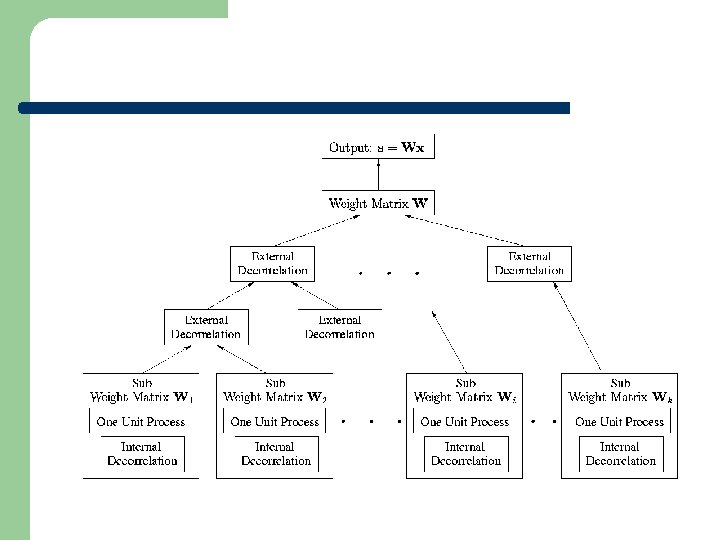
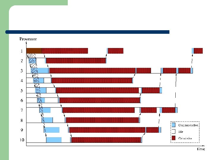
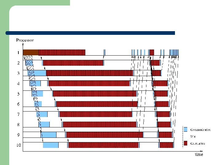
Model for p. ICA l Features – – – l SIMD High volume data set transfer at first stage Low volume data transfer at other stages Combine BSP and Log. P models – Stage 1: l l – Pipeline: hyperspectral image transfer, one unit (weight vector) estimations Parallel: Internal decorrelations in sub-matrices Other stages: l Parallel: External decorrelations

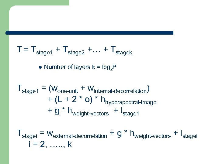T = Tstage 1 + Tstage 2 +… + Tstagek l Number of layers k = log 2 P Tstage 1 = (wone-unit + winternal-decorrelation) + (L + 2 * o) * hhyperspectral-image + g * hweight-vectors + lstage 1 Tstagei = wexternal-decorrelation + g * hweight-vectors + lstagei i = 2, …. . , k

Another Topic l Optimization of parallel computing – – – Heterogeneous parallel computing network Minimize overall time Tradeoff problem between computation (individual computer properties) and communication (network)

References l l l A. Hyv¨arinen and Erkki Oja, “A fast fixed-point algorithm for independent component analysis, ” Neural Computation, vol. 9, pp. 1483– 1492, 1997. P. Common, “Independent component analysis, a new concept, ” Signal Processing, vol. 36, no. 3, pp. 287– 314, April 1994, Special Issue on Highorder Statistics. A. J. Bell and T. J. Sejnowski, “An information maximisation approach to blind separation and blind deconvolution, ” Neural Computation, vol. 7, no. 6, pp. 1129– 1159, 1995. S. Amari, A. Cichochi, and H. Yang, “A new learning algorithm for blind signal separation, ” Advances in Neural Information Processing Systems, vol. 8, 1996. Te-Won Lee, Mark Girolami, Anthony J. Bell, and Terrence J. Sejnowski, “A unifying information-theoretic framework for independent component analysis, ” International Journal on Mathematical and Computer Modeling, 1998.