PACS Photometer Standard Pipeline Level 0 to Level

PACS Photometer Standard Pipeline Level 0 to Level 1 processing: From raw to calibrated data cubes - page 1 NHSC – DP workshop – Feb. 2011 – N. Billot

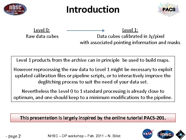Introduction Level 0: Raw data cubes PACS Level 1: Data cubes calibrated in Jy/pixel with associated pointing information and masks Level 1 products from the archive can in principle be used to build maps. However reprocessing the raw data to Level 1 might be necessary to exploit updated calibration files or pipeline scripts, or to interactively improve the deglitching process to suit the need of your data set. Nevertheless the Level 0 to 1 standard processing is already close to optimum, and one should keep to a minimum modifications to the pipeline. This presentation is largely inspired by the online tutorial PACS-201. - page 2 NHSC – DP workshop – Feb. 2011 – N. Billot

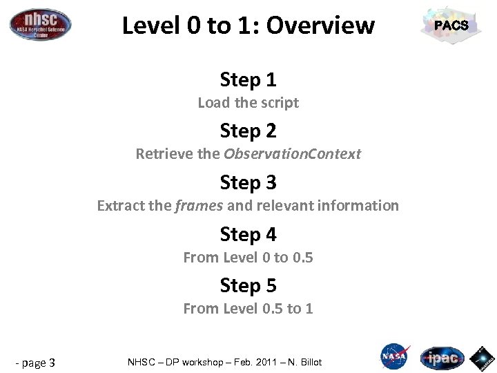Level 0 to 1: Overview Step 1 Load the script Step 2 Retrieve the Observation. Context Step 3 Extract the frames and relevant information Step 4 From Level 0 to 0. 5 Step 5 From Level 0. 5 to 1 - page 3 NHSC – DP workshop – Feb. 2011 – N. Billot PACS

PACS Step 1 Load the relevant data reduction script - page 4 NHSC – DP workshop – Feb. 2011 – N. Billot

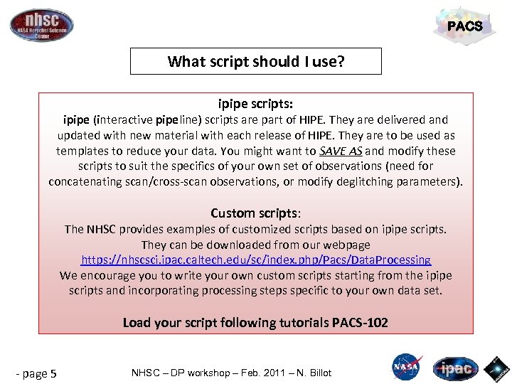PACS What script should I use? ipipe scripts: ipipe (interactive pipeline) scripts are part of HIPE. They are delivered and updated with new material with each release of HIPE. They are to be used as templates to reduce your data. You might want to SAVE AS and modify these scripts to suit the specifics of your own set of observations (need for concatenating scan/cross-scan observations, or modify deglitching parameters). Custom scripts: The NHSC provides examples of customized scripts based on ipipe scripts. They can be downloaded from our webpage https: //nhscsci. ipac. caltech. edu/sc/index. php/Pacs/Data. Processing We encourage you to write your own custom scripts starting from the ipipe scripts and incorporating processing steps specific to your own data set. Load your script following tutorials PACS-102 - page 5 NHSC – DP workshop – Feb. 2011 – N. Billot

PACS Step 2 Retrieve the Observation. Context - page 6 NHSC – DP workshop – Feb. 2011 – N. Billot

PACS Observation. Context: HIPE variable holding entire Herschel observations. It contains the raw data cube as well as the data processed with the standard pipeline up to Level 0. 5, 1 and 2. It also contains auxiliary information such as the telescope pointing, and all the calibration files necessary to reprocess the data. Definition of Observation Content: Herschel Data Analysis Guide Section 1. 2. 3 - page 7 NHSC – DP workshop – Feb. 2011 – N. Billot

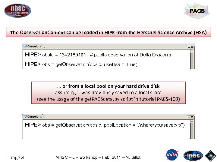PACS The Observation. Context can be loaded in HIPE from the Herschel Science Archive (HSA) HIPE> obsid = 1342189191 # public observation of Delta Draconis HIPE> obs = get. Observation(obsid, use. Hsa = True) … or from a local pool on your hard drive disk assuming it was previously saved to a local store (see the usage of the get. PACSdata. py script in tutorial PACS-103) HIPE> obs = get. Observation(obsid, pool. Location = “/where/you/saved/it/”) - page 8 NHSC – DP workshop – Feb. 2011 – N. Billot

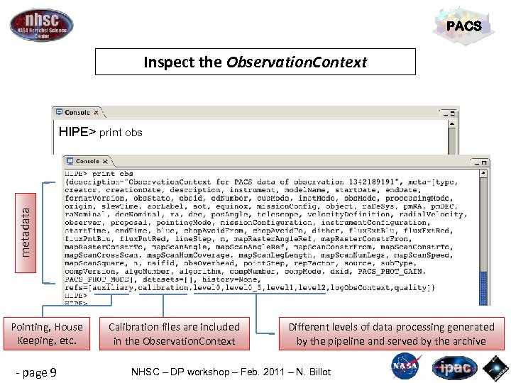PACS Inspect the Observation. Context metadata HIPE> print obs Pointing, House Keeping, etc. - page 9 Calibration files are included in the Observation. Context Different levels of data processing generated by the pipeline and served by the archive NHSC – DP workshop – Feb. 2011 – N. Billot

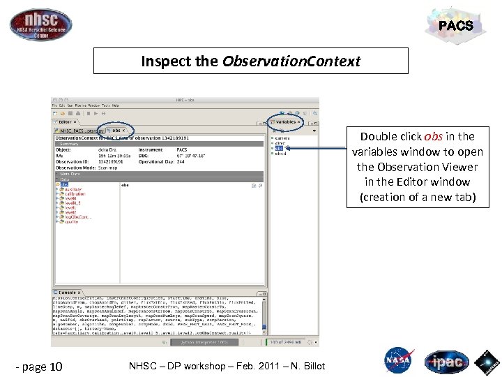PACS Inspect the Observation. Context Double click obs in the variables window to open the Observation Viewer in the Editor window (creation of a new tab) - page 10 NHSC – DP workshop – Feb. 2011 – N. Billot

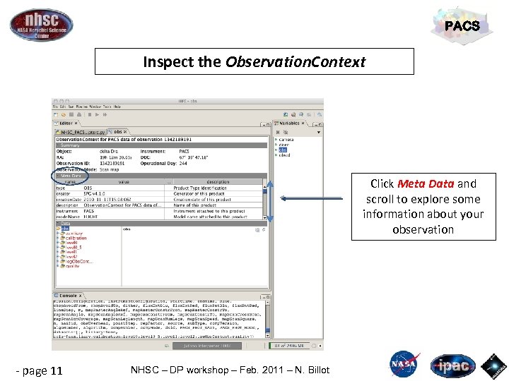PACS Inspect the Observation. Context Click Meta Data and scroll to explore some information about your observation - page 11 NHSC – DP workshop – Feb. 2011 – N. Billot

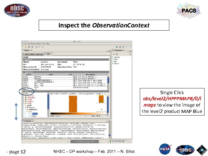PACS Inspect the Observation. Context Single Click obs/level 2/HPPPMAPB/0/i mage to view the image of the level 2 product MAP Blue - page 12 NHSC – DP workshop – Feb. 2011 – N. Billot

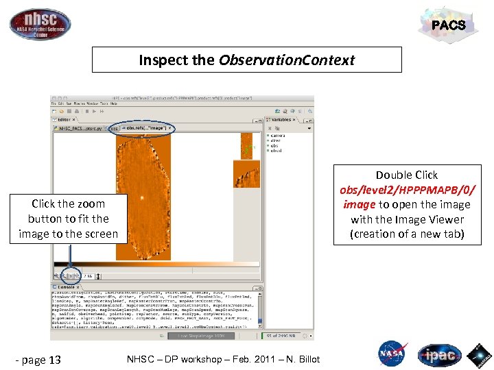PACS Inspect the Observation. Context Double Click obs/level 2/HPPPMAPB/0/ image to open the image with the Image Viewer (creation of a new tab) Click the zoom button to fit the image to the screen - page 13 NHSC – DP workshop – Feb. 2011 – N. Billot

PACS Step 3 Extract the frames and related information from the Observation. Context and HIPE - page 14 NHSC – DP workshop – Feb. 2011 – N. Billot

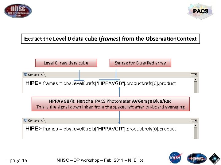PACS Extract the Level 0 data cube (frames) from the Observation. Context Level 0: raw data cube Syntax for Blue/Red array HIPE> frames = obs. level 0. refs["HPPAVGB"]. product. refs[0]. product HPPAVGB/R: Herschel PACS Photometer AVGerage Blue/Red This is the signal downlinked from the spacecraft after on-board averaging HIPE> frames = obs. level 0. refs["HPPAVGR"]. product. refs[0]. product - page 15 NHSC – DP workshop – Feb. 2011 – N. Billot

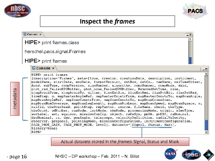PACS Inspect the frames HIPE> print frames. class herschel. pacs. signal. Frames metadata HIPE> print frames Actual datasets stored in the frames: Signal, Status and Mask - page 16 NHSC – DP workshop – Feb. 2011 – N. Billot

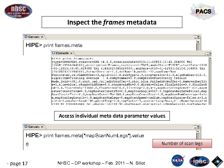PACS Inspect the frames metadata HIPE> print frames. meta Access individual meta data parameter values HIPE> print frames. meta["map. Scan. Num. Legs"]. value Number of scan legs 8 - page 17 NHSC – DP workshop – Feb. 2011 – N. Billot

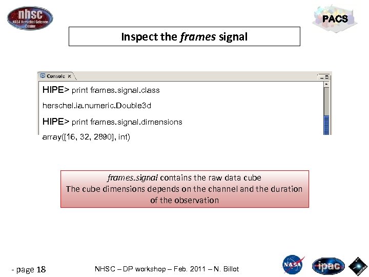PACS Inspect the frames signal HIPE> print frames. signal. class herschel. ia. numeric. Double 3 d HIPE> print frames. signal. dimensions array([16, 32, 2890], int) frames. signal contains the raw data cube The cube dimensions depends on the channel and the duration of the observation - page 18 NHSC – DP workshop – Feb. 2011 – N. Billot

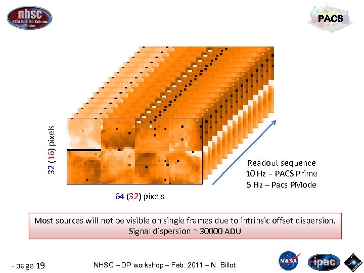32 (16) pixels PACS Readout sequence 10 Hz − PACS Prime 5 Hz – Pacs PMode 64 (32) pixels Most sources will not be visible on single frames due to intrinsic offset dispersion. Signal dispersion ~ 30000 ADU - page 19 NHSC – DP workshop – Feb. 2011 – N. Billot

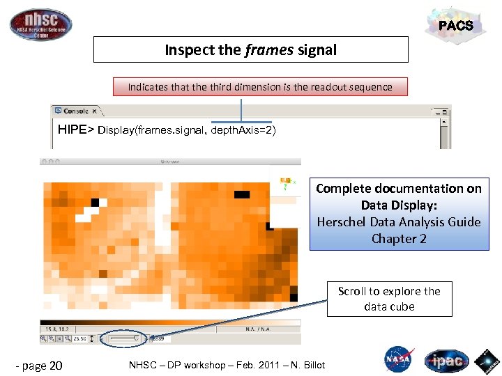PACS Inspect the frames signal Indicates that the third dimension is the readout sequence HIPE> Display(frames. signal, depth. Axis=2) Complete documentation on Data Display: Herschel Data Analysis Guide Chapter 2 Scroll to explore the data cube - page 20 NHSC – DP workshop – Feb. 2011 – N. Billot

PACS Inspect the frames signal HIPE> Plot. XY(frames. signal[8, 8, : ]) Temporal evolution of pixel (8, 8) Calibration Block: prior to any observations, 2 internal sources are observed with the internal chopper for calibration purposes Science Block Complete documentation on Data Plotting: Herschel Data Analysis Guide Chapter 3 - page 21 NHSC – DP workshop – Feb. 2011 – N. Billot

PACS Inspect the frames signal HIPE> Plot. XY(frames. signal[8, 8, : ]) Temporal evolution of pixel (8, 8) Zoom onto the Calibration Block Chopping pattern on internal sources 1 & 2 Complete documentation on Data Plotting: Herschel Data Analysis Guide Chapter 3 - page 22 NHSC – DP workshop – Feb. 2011 – N. Billot

PACS Inspect the frames signal HIPE> Plot. XY(frames. signal[8, 8, : ]) Temporal evolution of pixel (8, 8) Zoom onto the Science Block The spike is likely a glitch Complete documentation on Data Plotting: Herschel Data Analysis Guide Chapter 3 - page 23 NHSC – DP workshop – Feb. 2011 – N. Billot

PACS Inspect the frames signal HIPE> Plot. XY(frames. signal[8, 8, : ]) Temporal evolution of pixel (8, 8) Zoom onto the spike The spike is asymmetric and affects only 2 readouts: It is a glitch Complete documentation on Data Plotting: Herschel Data Analysis Guide Chapter 3 - page 24 NHSC – DP workshop – Feb. 2011 – N. Billot

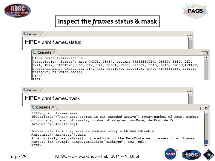PACS Inspect the frames status & mask HIPE> print frames. status HIPE> print frames. mask - page 25 NHSC – DP workshop – Feb. 2011 – N. Billot

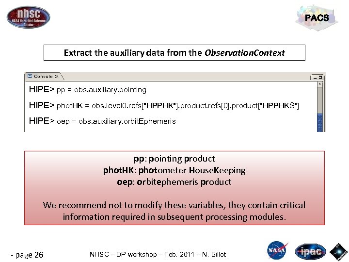PACS Extract the auxiliary data from the Observation. Context HIPE> pp = obs. auxiliary. pointing HIPE> phot. HK = obs. level 0. refs["HPPHK"]. product. refs[0]. product["HPPHKS"] HIPE> oep = obs. auxiliary. orbit. Ephemeris pp: pointing product phot. HK: photometer House. Keeping oep: orbitephemeris product We recommend not to modify these variables, they contain critical information required in subsequent processing modules. - page 26 NHSC – DP workshop – Feb. 2011 – N. Billot

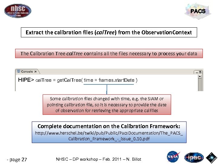PACS Extract the calibration files (cal. Tree) from the Observation. Context The Calibration Tree cal. Tree contains all the files necessary to process your data HIPE> cal. Tree = get. Cal. Tree( time = frames. start. Date ) Some calibration files changed with time, e. g. the SIAM or pointing calibration file, so it is necessary to provide the date of observation for retrieving the appropriate cal. Files Complete documentation on the Calibration Framework: http: //www. herschel. be/twiki/pub/Public/Pacs. Documentation/The_PACS_ Calibration_Framework_-_issue_0. 10. pdf - page 27 NHSC – DP workshop – Feb. 2011 – N. Billot

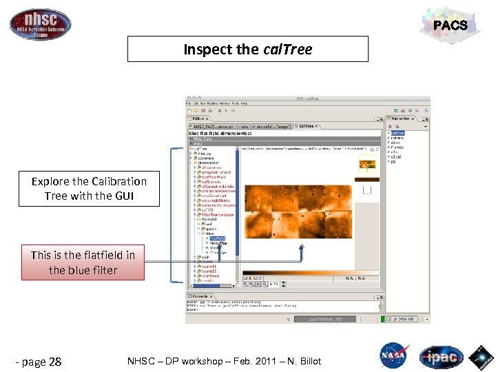PACS Inspect the cal. Tree Explore the Calibration Tree with the GUI This is the flatfield in the blue filter - page 28 NHSC – DP workshop – Feb. 2011 – N. Billot

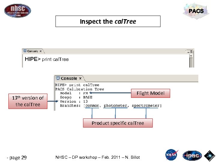PACS Inspect the cal. Tree HIPE> print cal. Tree 13 th version of the cal. Tree Flight Model Product specific cal. Tree - page 29 NHSC – DP workshop – Feb. 2011 – N. Billot

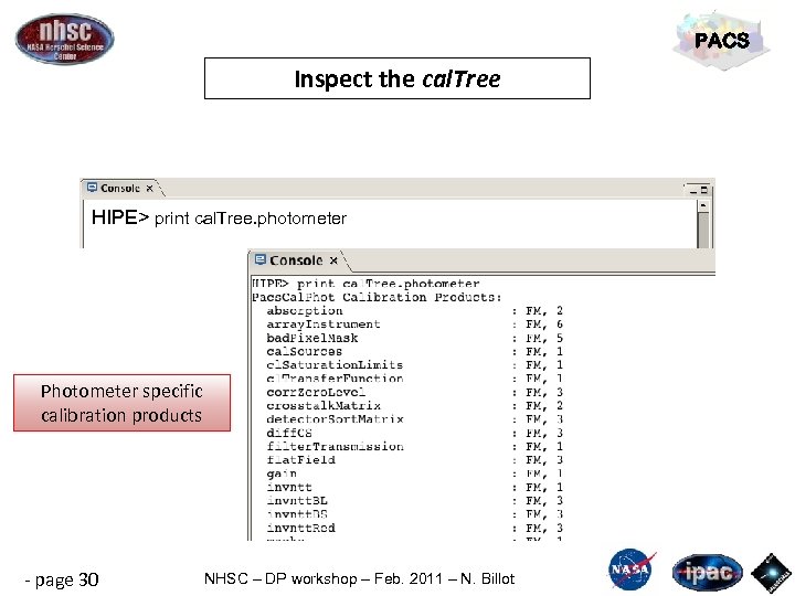PACS Inspect the cal. Tree HIPE> print cal. Tree. photometer Photometer specific calibration products - page 30 NHSC – DP workshop – Feb. 2011 – N. Billot

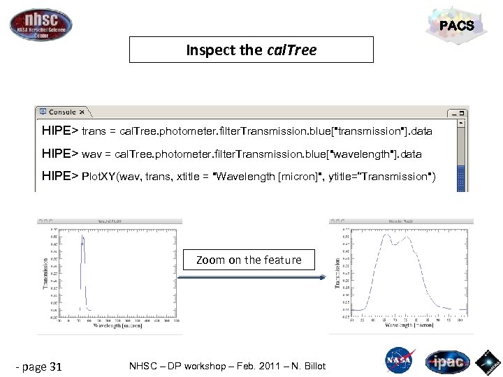PACS Inspect the cal. Tree HIPE> trans = cal. Tree. photometer. filter. Transmission. blue["transmission"]. data HIPE> wav = cal. Tree. photometer. filter. Transmission. blue["wavelength"]. data HIPE> Plot. XY(wav, trans, xtitle = "Wavelength [micron]", ytitle=“Transmission") Zoom on the feature - page 31 NHSC – DP workshop – Feb. 2011 – N. Billot

PACS Step 4 From Level-0 to Level-0. 5 - page 32 NHSC – DP workshop – Feb. 2011 – N. Billot

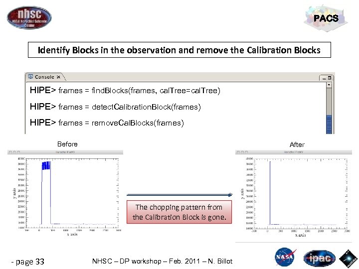PACS Identify Blocks in the observation and remove the Calibration Blocks HIPE> frames = find. Blocks(frames, cal. Tree=cal. Tree) HIPE> frames = detect. Calibration. Block(frames) HIPE> frames = remove. Cal. Blocks(frames) Before After The chopping pattern from the Calibration Block is gone. - page 33 NHSC – DP workshop – Feb. 2011 – N. Billot

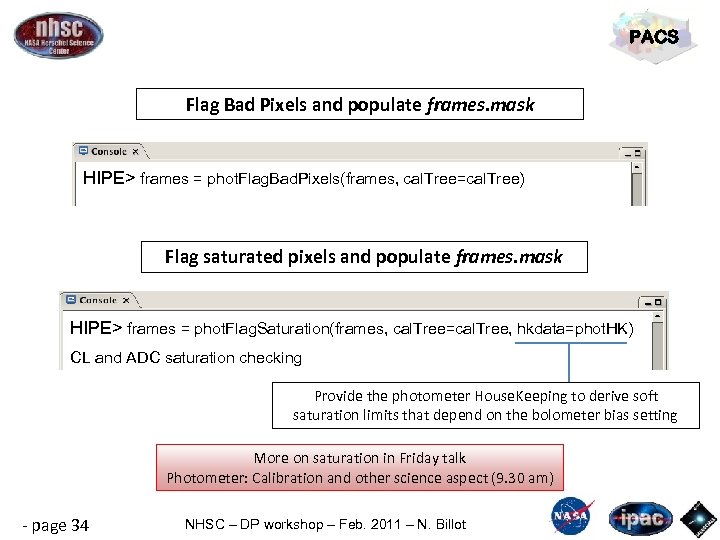PACS Flag Bad Pixels and populate frames. mask HIPE> frames = phot. Flag. Bad. Pixels(frames, cal. Tree=cal. Tree) Flag saturated pixels and populate frames. mask HIPE> frames = phot. Flag. Saturation(frames, cal. Tree=cal. Tree, hkdata=phot. HK) CL and ADC saturation checking Provide the photometer House. Keeping to derive soft saturation limits that depend on the bolometer bias setting More on saturation in Friday talk Photometer: Calibration and other science aspect (9. 30 am) - page 34 NHSC – DP workshop – Feb. 2011 – N. Billot

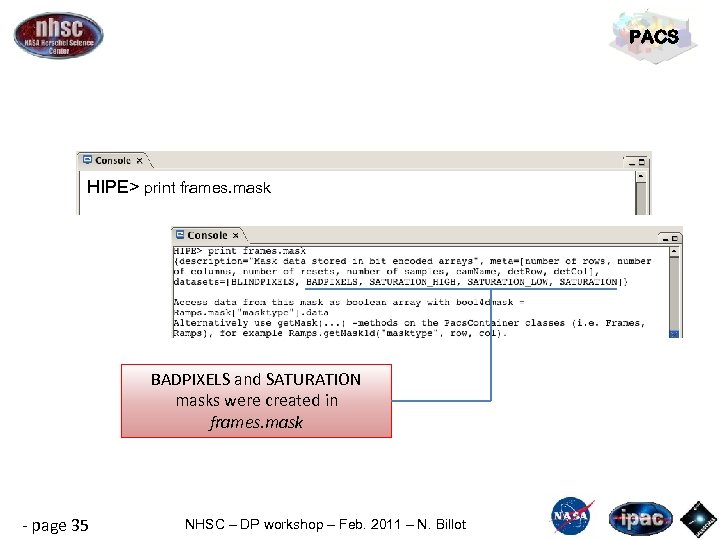PACS HIPE> print frames. mask BADPIXELS and SATURATION masks were created in frames. mask - page 35 NHSC – DP workshop – Feb. 2011 – N. Billot

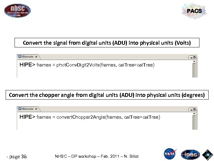PACS Convert the signal from digital units (ADU) into physical units (Volts) HIPE> frames = phot. Conv. Digit 2 Volts(frames, cal. Tree=cal. Tree) Convert the chopper angle from digital units (ADU) into physical units (degrees) HIPE> frames = convert. Chopper 2 Angle(frames, cal. Tree=cal. Tree) - page 36 NHSC – DP workshop – Feb. 2011 – N. Billot

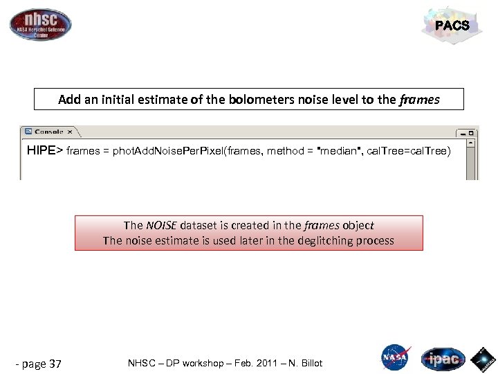PACS Add an initial estimate of the bolometers noise level to the frames HIPE> frames = phot. Add. Noise. Per. Pixel(frames, method = "median", cal. Tree=cal. Tree) The NOISE dataset is created in the frames object The noise estimate is used later in the deglitching process - page 37 NHSC – DP workshop – Feb. 2011 – N. Billot

PACS Step 5 From Level-0. 5 to Level-1 - page 38 NHSC – DP workshop – Feb. 2011 – N. Billot

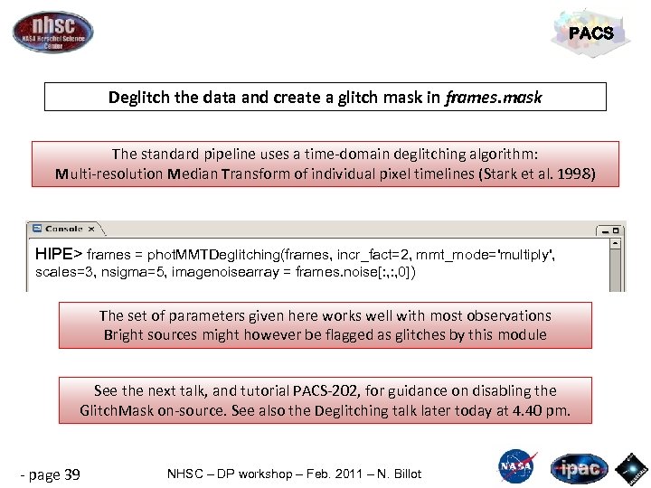PACS Deglitch the data and create a glitch mask in frames. mask The standard pipeline uses a time-domain deglitching algorithm: Multi-resolution Median Transform of individual pixel timelines (Stark et al. 1998) HIPE> frames = phot. MMTDeglitching(frames, incr_fact=2, mmt_mode='multiply', scales=3, nsigma=5, imagenoisearray = frames. noise[: , 0]) The set of parameters given here works well with most observations Bright sources might however be flagged as glitches by this module See the next talk, and tutorial PACS-202, for guidance on disabling the Glitch. Mask on-source. See also the Deglitching talk later today at 4. 40 pm. - page 39 NHSC – DP workshop – Feb. 2011 – N. Billot

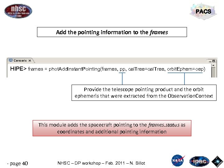PACS Add the pointing information to the frames HIPE> frames = phot. Add. Instant. Pointing(frames, pp, cal. Tree=cal. Tree, orbit. Ephem=oep) Provide the telescope pointing product and the orbit ephemeris that were extracted from the Observation. Context This module adds the spacecraft pointing to the frames. status as coordinates and additional pointing information - page 40 NHSC – DP workshop – Feb. 2011 – N. Billot

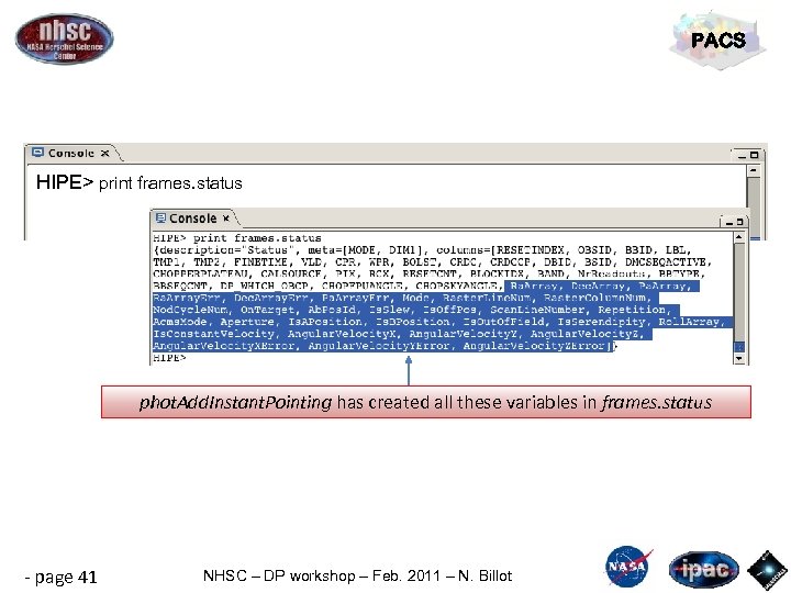PACS HIPE> print frames. status phot. Add. Instant. Pointing has created all these variables in frames. status - page 41 NHSC – DP workshop – Feb. 2011 – N. Billot

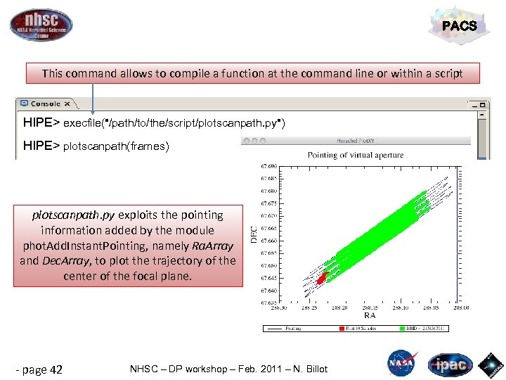PACS This command allows to compile a function at the command line or within a script HIPE> execfile("/path/to/the/script/plotscanpath. py") HIPE> plotscanpath(frames) plotscanpath. py exploits the pointing information added by the module phot. Add. Instant. Pointing, namely Ra. Array and Dec. Array, to plot the trajectory of the center of the focal plane. - page 42 NHSC – DP workshop – Feb. 2011 – N. Billot

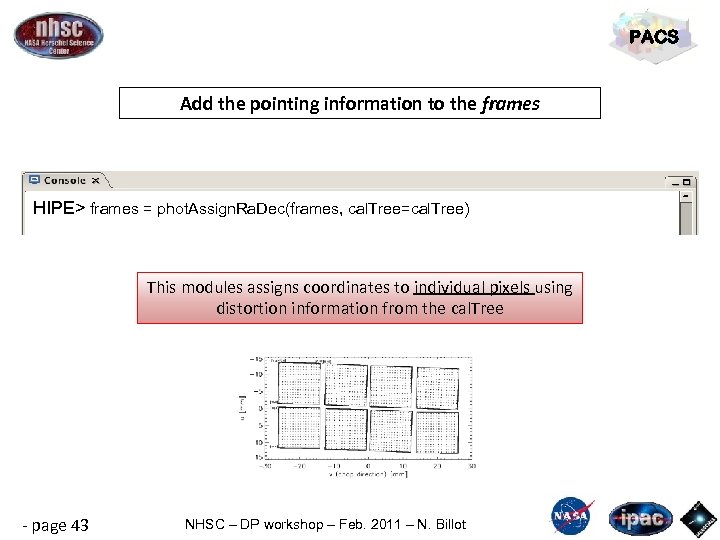PACS Add the pointing information to the frames HIPE> frames = phot. Assign. Ra. Dec(frames, cal. Tree=cal. Tree) This modules assigns coordinates to individual pixels using distortion information from the cal. Tree - page 43 NHSC – DP workshop – Feb. 2011 – N. Billot

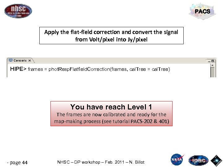PACS Apply the flat-field correction and convert the signal from Volt/pixel into Jy/pixel HIPE> frames = phot. Resp. Flatfield. Correction(frames, cal. Tree = cal. Tree) You have reach Level 1 The frames are now calibrated and ready for the map-making process (see tutorial PACS-202 & 401) - page 44 NHSC – DP workshop – Feb. 2011 – N. Billot

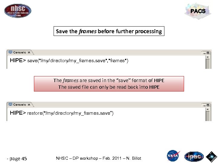PACS Save the frames before further processing HIPE> save("/my/directory/my_frames. save", "frames") The frames are saved in the “save” format of HIPE The saved file can only be read back into HIPE> restore("/my/directory/my_frames. save”) - page 45 NHSC – DP workshop – Feb. 2011 – N. Billot

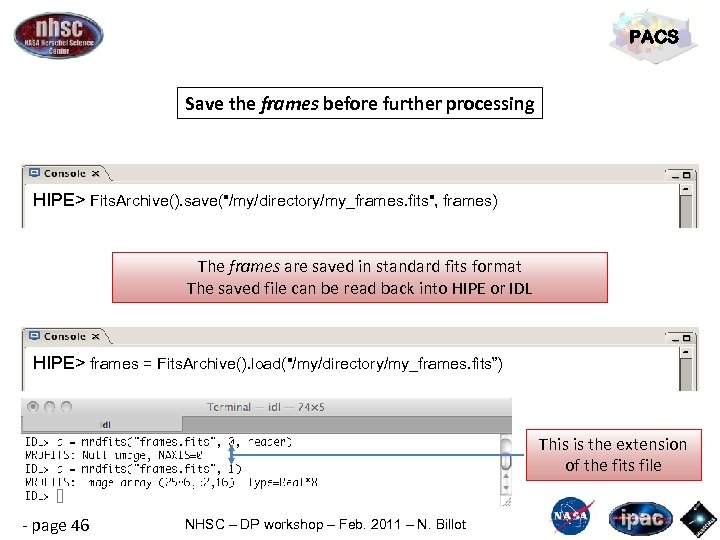PACS Save the frames before further processing HIPE> Fits. Archive(). save("/my/directory/my_frames. fits", frames) The frames are saved in standard fits format The saved file can be read back into HIPE or IDL HIPE> frames = Fits. Archive(). load("/my/directory/my_frames. fits”) This is the extension of the fits file - page 46 NHSC – DP workshop – Feb. 2011 – N. Billot

Documentation PACS http: //herschel. esac. esa. int/hcss-doc-5. 0/ http: //www. herschel. be/twiki/bin/view/Public/ Most relevant documentation for this tutorial: • PACS Data Reduction Guide • PACS User’s Reference Manual • HCSS User’s Reference Manual General documentation necessary to manipulate the data: • HIPE Owner’s Guide • Herschel Data Analysis Guide • Scripting and Data Mining - page 47 NHSC – DP workshop – Feb. 2011 – N. Billot