Overview u Demand u Supply u Underlying principles

Overview u. Demand u. Supply u. Underlying principles u. Factors impacting supply and demand u. Special S&D curves u. Chapter 4 in text

Demand u. Various quantities of a commodity that an individual is willing and able to buy as the price of the commodity varies holding all other factors constant.

Law of Demand u. All else equal consumers will by more of a item at lower prices and buy less at higher prices. u. Demand begins with individual consumer u. Inverse relationship between quantity and price • Two dimensional, Price and Quantity

Downward Sloping Demand Curve Px A PA B PB D QA QB Qx

Downward sloping demand u. Begin with individual’s utility function and a budget constraint u. Substitution effect • consumers buy what’s cheaper u. Income effect • “income” increases if prices fall

Representation of Demand P Q $6. 00 2. 0 $5. 00 4. 0 $4. 00 6. 0 $3. 00 8. 0 $2. 00 10. 0 $1. 00 12. 0 Q = 14 – 2 x. P P Q

Market or Aggregate Demand u. Add individual demand curves u. Horizontally across consumers uhttp: //www. aaec. vt. edu/rilp/Demand% 20 Changes-2000. pdf (Pages 1 -10)

Aggregate Demand u. Add horizontally across consumers at each price 1 2 3 Market

Change in Demand or in Quantity Demanded Px A Moving from A to B due to a price decline is a change in quantity demanded by moving along the same demand curve. A shift in demand is a move from B to C as the curve shifts from D 1 to D 2 B C D 1 D 2 Qx

Factors that Cause a Shift in Demand u. Price of substitutes u. Price of complements u. Consumer income u. Taste and preferences u. IS NOT FUNCTION OF THE GOOD’S OWN PRICE

Factors that cause a shift in aggregate demand u Population u Exports u Consumer income u Advertising u New information u Product differentiation u New product development u Government intervention

Observing Demand in Data u. Each P and Q are an equilibrium point where supply equals demand at a point in time. u. Demand typically more stable u. As supply changes the demand curve is traced out

US Corn Price, 1995 -96 to 2004 -05 Crop Years Crop Year 1995 -96 1996 -97 1997 -98 Quantity 8974 9672 10099 Price 3. 24 2. 71 2. 43 1998 -99 1999 -00 2000 -01 2001 -02 2002 -03 2003 -04 2004 -05 11085 11232 11639 11416 10578 11190 12780 1. 94 1. 82 1. 85 1. 97 2. 32 2. 42 1. 95

US Corn Price, 1995 -96 to 2004 -05 Crop Years

US Soybean Price, 1996 -97 to 2004 -05 Crop Years Crop Year 1996 -97 1997 -98 Quantity 2573 2826 Price 7. 35 6. 47 1998 -99 1999 -00 2000 -01 2001 -02 2002 -03 2003 -04 2004 -05 2945 3006 3052 3140 2969 2638 3258 4. 93 4. 63 4. 54 4. 38 5. 53 7. 34 5. 54

US Soybean Price, 1996 -97 to 2004 -05 Crop Years

Per Capita Consumption in Pounds

Per Capita Consumption in Pounds

Inverse Demand u. Price is a function of quantity • P = f(Q) u. Important in agriculture • Short run supplies are relatively fixed • Prices change to clear the market

Supply u. The amount of a given commodity that will be offered for sale per unit time as the price varies, other factors held constant.

Law of Supply u. An economic principle that states: All else equal, producers are willing to sell more products at a higher price than at a lower one. u. Positive relationship between price and quantity u. Curve slopes up and to the right

Supply u. Derived from cost function • Production function • Input - output relationship u. Assume that firms seek to • Maximize profits • Minimize costs u. Supply starts will individual firm

Production Function Output Total Product Decreasing returns to the input Input

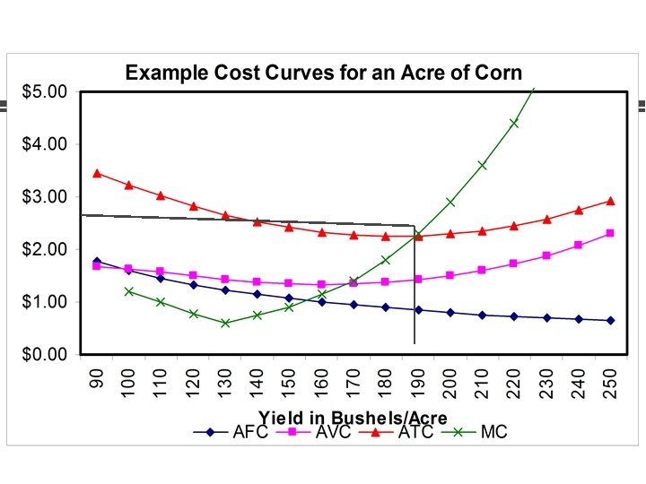
Cost Curves u. Average variable cost = AVC • Total variable cost / Q • Total variable costs change with Q u. Average fixed cost = AFC • Total fixed cost / Q • Total fixed costs do not change with Q u. Average total cost = ATC = AVC+AFC

Cost Curves u. Marginal cost = MC • Change in total cost by producing 1 more • TC / Q

Cost curves Cost MC ATC AVC AFC Q

Profit for the firm u. Profit = total revenue - total cost • TR= P x Q • TC = ATC x Q u. Profit per unit = Profit/Q • = TR/Q - TC/Q • = P - ATC u. Profit maximizing Q • MC=MR=P • Profit/Q = P-ATC at optimal Q

Optimal Q at P=MC Cost MC P 2 ATC AVC P 1 Q 2 Q

Cost curves and supply u. Operate if ATC > P > AVC u. Shut down if P < AVC • Lose on every unit produced • P>AVC make some payment to fixed cost u. In the long run everything is variable • Short run defined by having fixed cost u. Long run supply curve for individual • Low point on ATC curve

Supply curve u. MC curve above AVC curve u. Upward sloping curve • • • Optimal output @ MC = MR MR = Price => Optimal at MC=Price The last unit of input just pays for itself – The change in the cost of the last unit is equal to the change in revenue of the last unit.

Example Cost Curves for Corn Units Fixed Variable Total AFC AVC ATC MC 130 160 186 346 1. 23 1. 43 2. 66 0. 60 140 160 193 353 1. 14 1. 38 2. 52 0. 75 150 160 202 362 1. 07 1. 35 2. 41 0. 90 160 214 374 1. 00 1. 34 2. 34 1. 15 170 160 228 388 0. 94 1. 34 2. 28 1. 40 180 160 246 406 0. 89 1. 37 2. 25 1. 80 190 160 269 429 0. 84 1. 41 2. 26 2. 30 200 160 298 458 0. 80 1. 49 2. 29 2. 90 210 160 334 494 0. 76 1. 59 2. 35 3. 60 220 160 378 538 0. 73 1. 72 2. 44 4. 40 230 160 433 593 0. 70 1. 88 2. 58 5. 50 240 160 498 658 0. 67 2. 07 2. 74 6. 50 250 160 574 734 0. 64 2. 29 2. 93 7. 60

Market or Aggregate Supply u. Combination of individual supply schedules • Add horizontally across firms A B C Market

Market supply curves Px A S 1 S 2 Move from A to B is a change in quantity supplied due to a price decline. B C Move from B to C is a shift in supply. Qx

Supply Shifts from Change uin input prices uin returns for competing enterprises uin price of joint products uin technology on yields or costs uin yield and/or price risk uinstitutional constraints u. SUPPLY DOES NOT CHANGE DUE TO A CHANGE IN PRICE OF THE OUTPUT

Following Supply Shift u. Firm level decision to supply shifter u. Market impact of firms’ decision u. Firm response to price reaction

Supply Shift from Cost S 1 MC 2 S 2 MC 1 P 2 D Q 1 Firm Q 2 Q Q 1 Market Q 2 Q

Steps to shift curves 1. 2. 3. 4. 5. The impact changes the MC curve of the firm. The firm chooses output so that MC = MR. Market supply shifts. Price moves along demand curve to new level. Repeat steps 2 - 4.

Market supply curves flatten out over time Px SShort run SLong run Qx

Price and Costs in Ag u. Short run • Not necessarily a relationship between cost and price • May be profit or loss u. Long run • Firms expand output to profits and reduce output to losses • Average price = Minimum Long Run ATC

Economies of scale Average total costs changes as the output of a firm changes u Increasing, decreasing or constant economies of scale. u • • Short run cost curve (SRATC) Long run cost curve (LRATC) Change across range u L-Shaped cost curve u

Externalities and cost curves Cost u. Cost or benefit not perceived by the firm u. Internal cost curve u. Cost curve if external cost included Q

Processing cost curves u. Specialized plants/equipment u. High fixed cost Cost u. Low flexibility SRATC Q

Law of One Price Definition: Under competitive market conditions all prices within a market are uniform after taking into account the cost of adding place, time, and form utility.

Marketing Adds Value u. Time utility: Storage u. Form utility: Processing u. Place utility: Transportation u. Does the added value offset the added cost? u. Is the cost the same for everyone?

Law of One Price u. Reason the Law of One Price Works: Arbitrage • Profit seeking individuals acting in their own self interest – Sellers, Buyers, Middlemen • Buy low and sell high for profit by changing time, space, and form

Law of One Price u. Arbitrage opportunities • Transportation • Storage • Processing u. How much price difference is sustainable between the two markets?

Seasonal Grain Prices u. Storable commodity u. One harvest period u. Used throughout the year

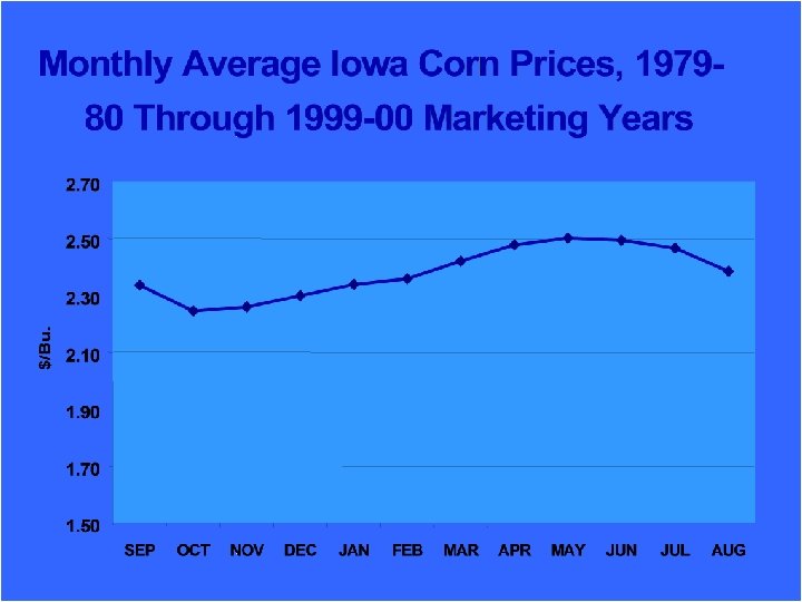
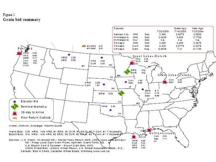
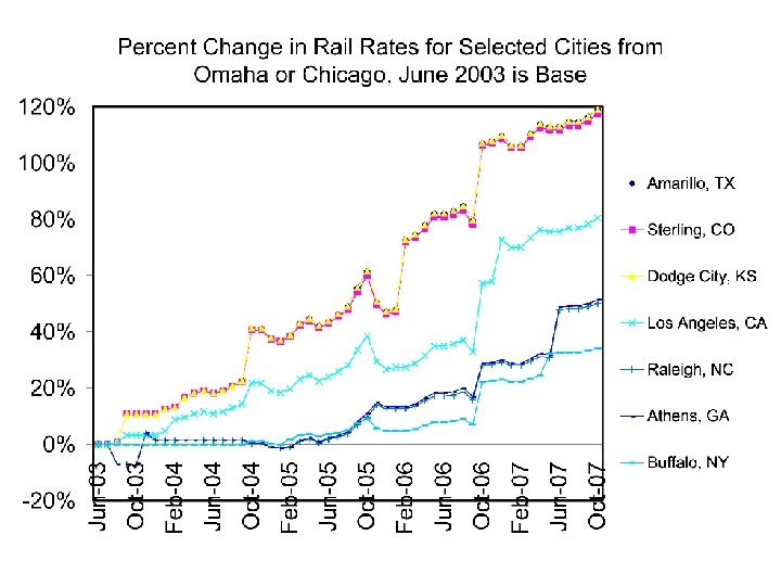
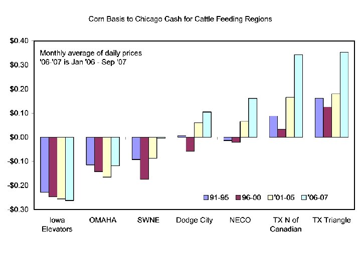
Transportation u. Products flow from surplus region to deficient region. u. Competing demand for surplus in some regions. u. Transportation infrastructure important

Aug 17, 2007 Corn Basis http: //www. card. iastate. edu/ag_risk_tools/

Aug 17, 2007 Corn Basis http: //www. card. iastate. edu/ag_risk_tools/

Grain Price Map CARD: Daily Corn and Soybean Basis Maps for Iowa

So what? ? ? u. Short run price implications u. Supply chain management u. Open market or contract • Packing plants • Ethanol plants • Soybean processing • Biodiesel