Overview on Classification and Clustering CENG 770 16

Overview on Classification and Clustering CENG 770 16 March 2018 1

Classification 16 March 2018 2

Classification vs. Prediction • Classification – predicts categorical class labels (discrete or nominal) – classifies data (constructs a model) based on the training set and the values (class labels) in a classifying attribute and uses it in classifying new data • Prediction – models continuous-valued functions, i. e. , predicts unknown or missing values 16 March 2018 3

Classification—A Two-Step Process • Model construction: describing a set of predetermined classes – Each tuple/sample is assumed to belong to a predefined class, as determined by the class label attribute – The set of tuples used for model construction is training set – The model is represented as classification rules, decision trees, or mathematical formulae • Model usage: for classifying future or unknown objects – Estimate accuracy of the model • The known label of test sample is compared with the classified result from the model • Accuracy rate is the percentage of test set samples that are correctly classified by the model • Test set is independent of training set, otherwise over-fitting will occur – If the accuracy is acceptable, use the model to classify data tuples whose class labels are not known 16 March 2018 4

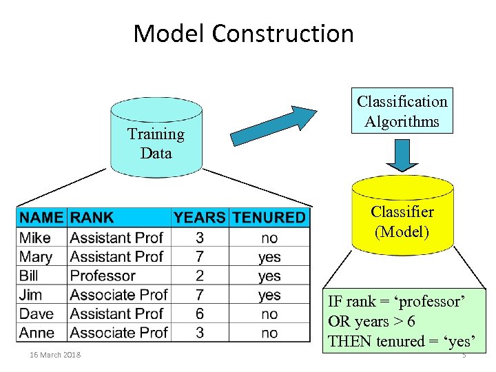Model Construction Training Data Classification Algorithms Classifier (Model) 16 March 2018 IF rank = ‘professor’ OR years > 6 THEN tenured = ‘yes’ 5

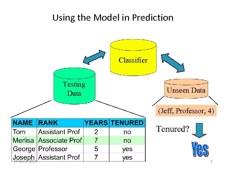Using the Model in Prediction Classifier Testing Data Unseen Data (Jeff, Professor, 4) Tenured? 16 March 2018 6

Classification Methods • • • Decision Tree Learning Bayesian Classification ANN SVM Lazy Learners 16 March 2018 7

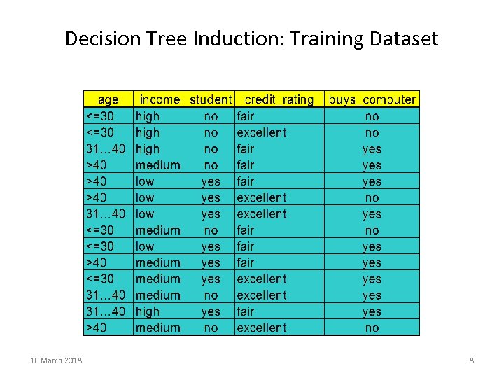Decision Tree Induction: Training Dataset 16 March 2018 8

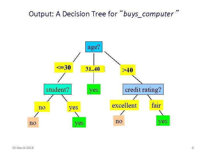Output: A Decision Tree for “buys_computer” age? <=30 31. . 40 overcast student? no no 16 March 2018 >40 credit rating? yes yes excellent no fair yes 9

Algorithm for Decision Tree Induction • Basic algorithm (a greedy algorithm) – Tree is constructed in a top-down recursive divide-and-conquer manner – At start, all the training examples are at the root – Attributes are categorical (if continuous-valued, they are discretized in advance) – Examples are partitioned recursively based on selected attributes – Test attributes are selected on the basis of a heuristic or statistical measure (e. g. , information gain) • Conditions for stopping partitioning – All samples for a given node belong to the same class – There are no remaining attributes for further partitioning – majority voting is employed for classifying the leaf – There are no samples left 16 March 2018 10

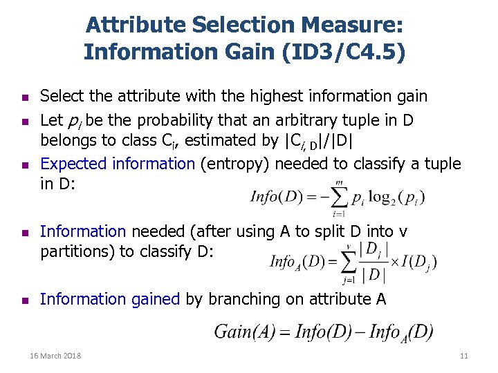Attribute Selection Measure: Information Gain (ID 3/C 4. 5) n n n Select the attribute with the highest information gain Let pi be the probability that an arbitrary tuple in D belongs to class Ci, estimated by |Ci, D|/|D| Expected information (entropy) needed to classify a tuple in D: Information needed (after using A to split D into v partitions) to classify D: Information gained by branching on attribute A 16 March 2018 11

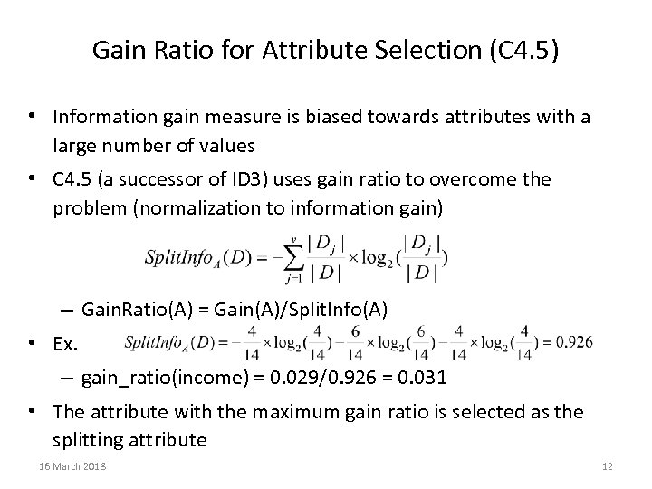Gain Ratio for Attribute Selection (C 4. 5) • Information gain measure is biased towards attributes with a large number of values • C 4. 5 (a successor of ID 3) uses gain ratio to overcome the problem (normalization to information gain) – Gain. Ratio(A) = Gain(A)/Split. Info(A) • Ex. – gain_ratio(income) = 0. 029/0. 926 = 0. 031 • The attribute with the maximum gain ratio is selected as the splitting attribute 16 March 2018 12

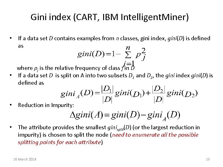Gini index (CART, IBM Intelligent. Miner) • If a data set D contains examples from n classes, gini index, gini(D) is defined as where pj is the relative frequency of class j in D • If a data set D is split on A into two subsets D 1 and D 2, the gini index gini(D) is defined as • Reduction in Impurity: • The attribute provides the smallest ginisplit(D) (or the largest reduction in impurity) is chosen to split the node (need to enumerate all the possible splitting points for each attribute) 16 March 2018 13

Bayesian Classification • A statistical classifier: performs probabilistic prediction, i. e. , predicts class membership probabilities • Foundation: Based on Bayes’ Theorem. • Performance: A simple Bayesian classifier, naïve Bayesian classifier, has comparable performance with decision tree and selected neural network classifiers • Incremental: Each training example can incrementally increase/decrease the probability that a hypothesis is correct — prior knowledge can be combined with observed data 16 March 2018 14

Bayesian Theorem: Basics • Let X be a data sample (“evidence”): class label is unknown • Let H be a hypothesis that X belongs to class C • Classification is to determine P(H|X), the probability that the hypothesis holds given the observed data sample X • P(H) (prior probability), the initial probability – E. g. , X will buy computer, regardless of age, income, … • P(X): probability that sample data is observed • P(X|H) (posteriori probability), the probability of observing the sample X, given that the hypothesis holds – E. g. , Given that X will buy computer, the prob. that X is 31. . 40, medium income 16 March 2018 15

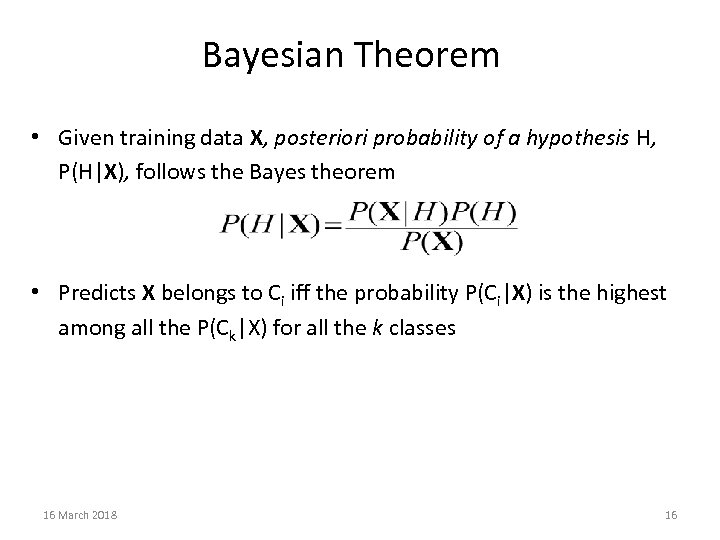Bayesian Theorem • Given training data X, posteriori probability of a hypothesis H, P(H|X), follows the Bayes theorem • Predicts X belongs to Ci iff the probability P(Ci|X) is the highest among all the P(Ck|X) for all the k classes 16 March 2018 16

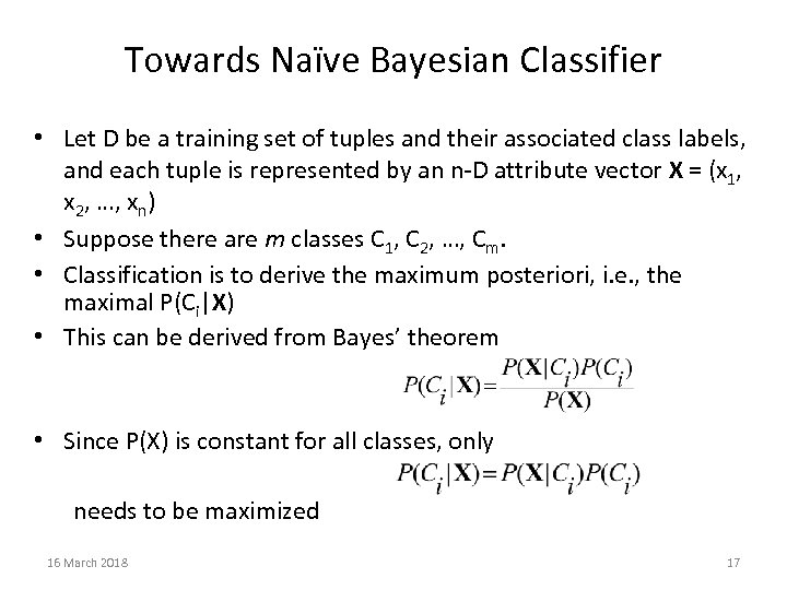Towards Naïve Bayesian Classifier • Let D be a training set of tuples and their associated class labels, and each tuple is represented by an n-D attribute vector X = (x 1, x 2, …, xn) • Suppose there are m classes C 1, C 2, …, Cm. • Classification is to derive the maximum posteriori, i. e. , the maximal P(Ci|X) • This can be derived from Bayes’ theorem • Since P(X) is constant for all classes, only needs to be maximized 16 March 2018 17

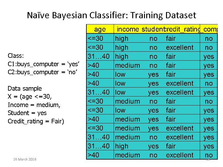Naïve Bayesian Classifier: Training Dataset Class: C 1: buys_computer = ‘yes’ C 2: buys_computer = ‘no’ Data sample X = (age <=30, Income = medium, Student = yes Credit_rating = Fair) 16 March 2018 18

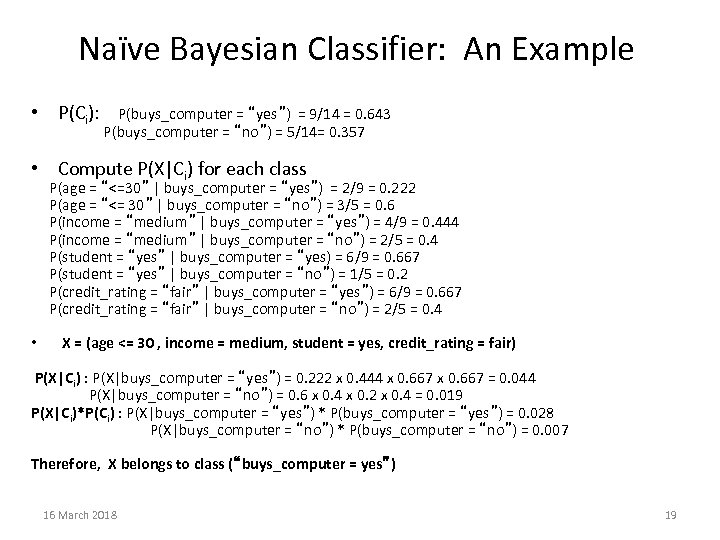Naïve Bayesian Classifier: An Example • P(Ci): P(buys_computer = “yes”) = 9/14 = 0. 643 P(buys_computer = “no”) = 5/14= 0. 357 • Compute P(X|Ci) for each class P(age = “<=30” | buys_computer = “yes”) = 2/9 = 0. 222 P(age = “<= 30” | buys_computer = “no”) = 3/5 = 0. 6 P(income = “medium” | buys_computer = “yes”) = 4/9 = 0. 444 P(income = “medium” | buys_computer = “no”) = 2/5 = 0. 4 P(student = “yes” | buys_computer = “yes) = 6/9 = 0. 667 P(student = “yes” | buys_computer = “no”) = 1/5 = 0. 2 P(credit_rating = “fair” | buys_computer = “yes”) = 6/9 = 0. 667 P(credit_rating = “fair” | buys_computer = “no”) = 2/5 = 0. 4 • X = (age <= 30 , income = medium, student = yes, credit_rating = fair) P(X|Ci) : P(X|buys_computer = “yes”) = 0. 222 x 0. 444 x 0. 667 = 0. 044 P(X|buys_computer = “no”) = 0. 6 x 0. 4 x 0. 2 x 0. 4 = 0. 019 P(X|Ci)*P(Ci) : P(X|buys_computer = “yes”) * P(buys_computer = “yes”) = 0. 028 P(X|buys_computer = “no”) * P(buys_computer = “no”) = 0. 007 Therefore, X belongs to class (“buys_computer = yes”) 16 March 2018 19

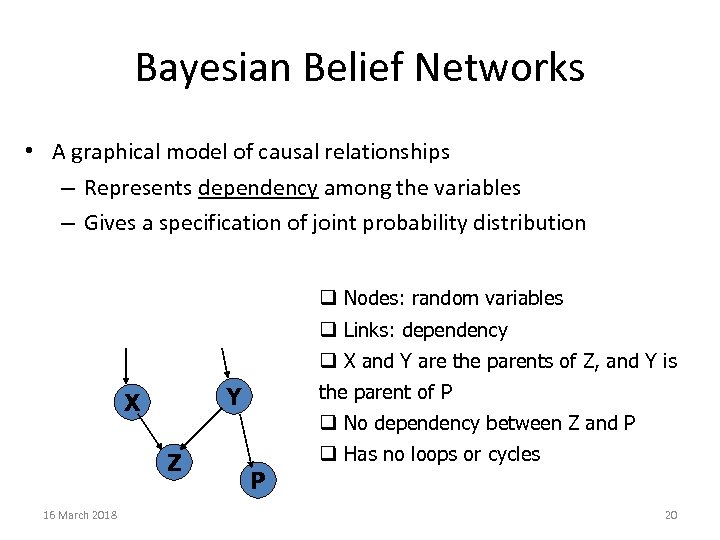Bayesian Belief Networks • A graphical model of causal relationships – Represents dependency among the variables – Gives a specification of joint probability distribution q Nodes: random variables q Links: dependency q X and Y are the parents of Z, and Y is Z 16 March 2018 the parent of P Y X q No dependency between Z and P P q Has no loops or cycles 20

Classification by Backpropagation • Backpropagation: A neural network learning algorithm • A neural network: A set of connected input/output units where each connection has a weight associated with it • During the learning phase, the network learns by adjusting the weights so as to be able to predict the correct class label of the input tuples • Also referred to as connectionist learning due to the connections between units 16 March 2018 21

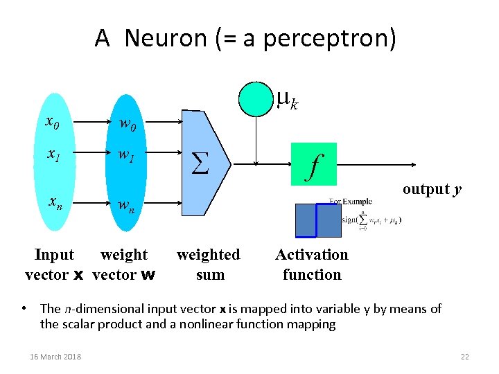A Neuron (= a perceptron) x 0 w 0 x 1 w 1 - mk xn å f wn Input weight vector x vector w weighted sum output y Activation function • The n-dimensional input vector x is mapped into variable y by means of the scalar product and a nonlinear function mapping 16 March 2018 22

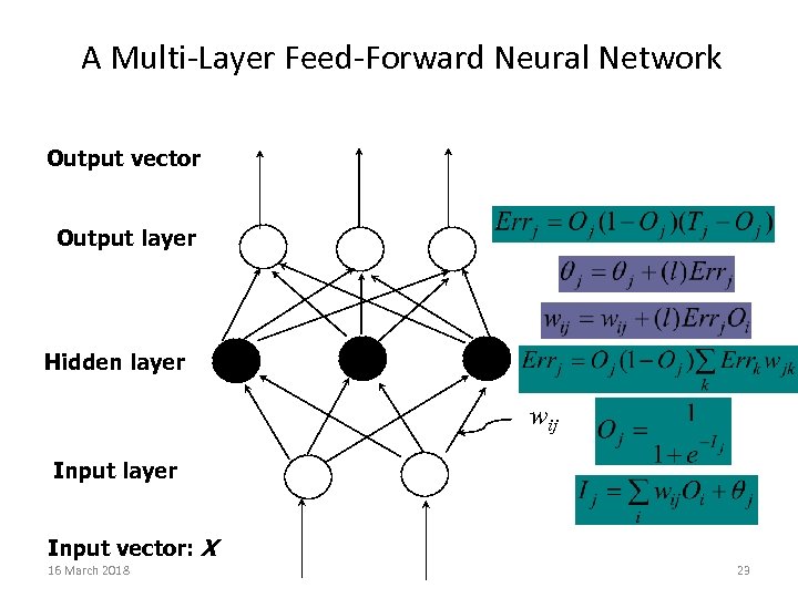A Multi-Layer Feed-Forward Neural Network Output vector Output layer Hidden layer wij Input layer Input vector: X 16 March 2018 23

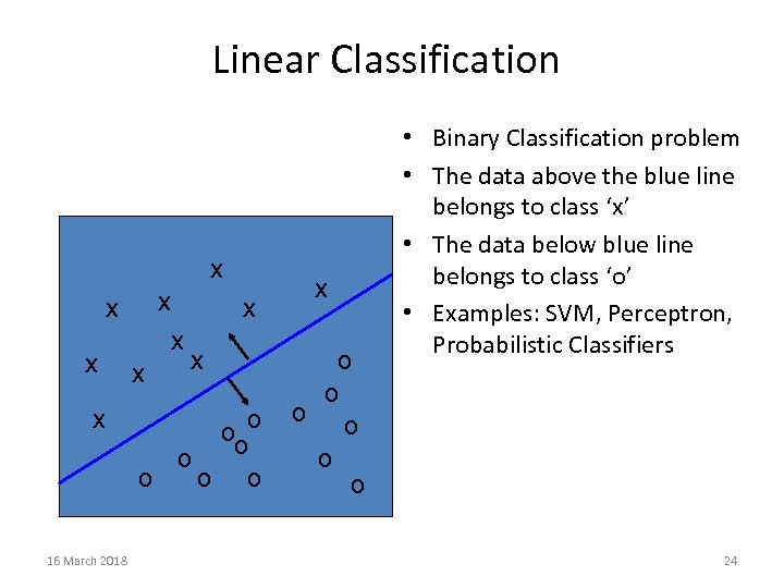Linear Classification x x x 16 March 2018 x x ooo o o x o o o • Binary Classification problem • The data above the blue line belongs to class ‘x’ • The data below blue line belongs to class ‘o’ • Examples: SVM, Perceptron, Probabilistic Classifiers 24

SVM—History and Applications • Vapnik and colleagues (1992)—groundwork from Vapnik & Chervonenkis’ statistical learning theory in 1960 s • Features: training can be slow but accuracy is high owing to their ability to model complex nonlinear decision boundaries (margin maximization) • Used both for classification and prediction 16 March 2018 25

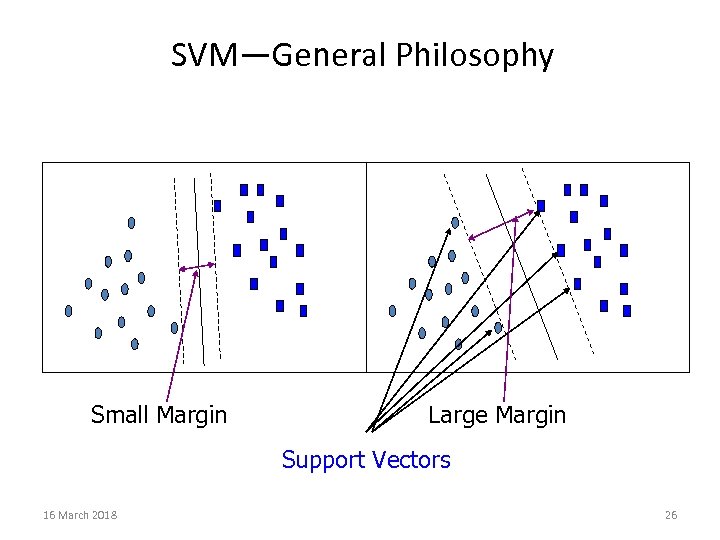SVM—General Philosophy Small Margin Large Margin Support Vectors 16 March 2018 26

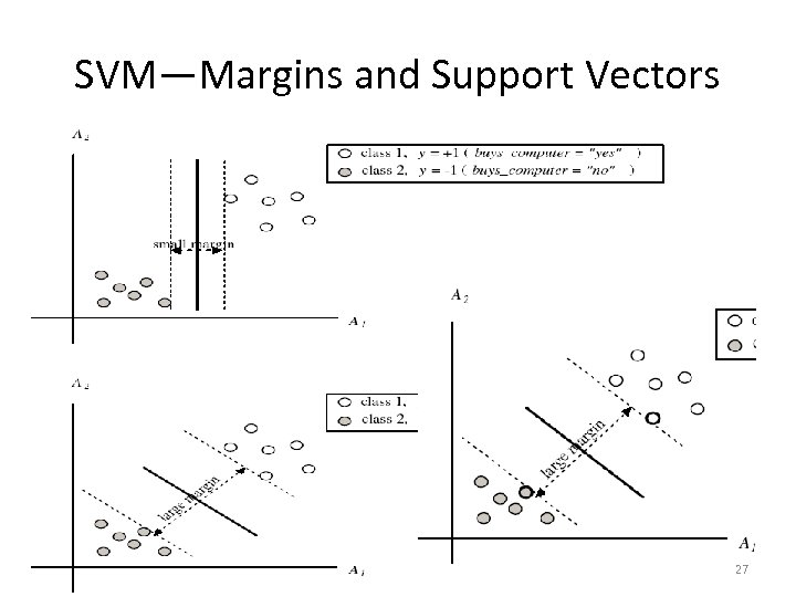SVM—Margins and Support Vectors 16 March 2018 27

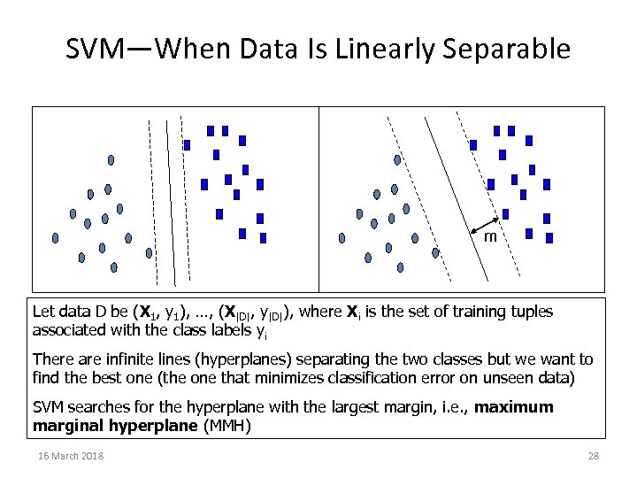SVM—When Data Is Linearly Separable m Let data D be (X 1, y 1), …, (X|D|, y|D|), where Xi is the set of training tuples associated with the class labels yi There are infinite lines (hyperplanes) separating the two classes but we want to find the best one (the one that minimizes classification error on unseen data) SVM searches for the hyperplane with the largest margin, i. e. , maximum marginal hyperplane (MMH) 16 March 2018 28

Lazy vs. Eager Learning • Lazy vs. eager learning – Lazy learning (e. g. , instance-based learning): Simply stores training data (or only minor processing) and waits until it is given a test tuple – Eager learning (the previously discussed methods): Given a set of training set, constructs a classification model before receiving new (e. g. , test) data to classify • Lazy: less time in training but more time in predicting 16 March 2018 29

Lazy Learner: Instance-Based Methods • Instance-based learning: – Store training examples and delay the processing (“lazy evaluation”) until a new instance must be classified • Typical approaches – k-nearest neighbor approach • Instances represented as points in a Euclidean space. – Case-based reasoning • Uses symbolic representations and knowledge-based inference 16 March 2018 30

The k-Nearest Neighbor Algorithm • All instances correspond to points in the n-D space • The nearest neighbor are defined in terms of Euclidean distance, dist(X 1, X 2) • For discrete-valued, k-NN returns the most common value among the k training examples nearest to xq 16 March 2018 31

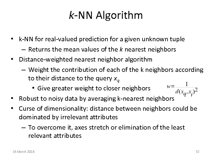k-NN Algorithm • k-NN for real-valued prediction for a given unknown tuple – Returns the mean values of the k nearest neighbors • Distance-weighted nearest neighbor algorithm – Weight the contribution of each of the k neighbors according to their distance to the query xq • Give greater weight to closer neighbors • Robust to noisy data by averaging k-nearest neighbors • Curse of dimensionality: distance between neighbors could be dominated by irrelevant attributes – To overcome it, axes stretch or elimination of the least relevant attributes 16 March 2018 32

What Is Prediction? • (Numerical) prediction is similar to classification – construct a model – use model to predict continuous or ordered value for a given input • Prediction is different from classification – Classification refers to predict categorical class label – Prediction models continuous-valued functions • Major method for prediction: regression – model the relationship between one or more independent or predictor variables and a dependent or response variable • Regression analysis – Linear and multiple regression – Non-linear regression – Other regression methods: generalized linear model, Poisson regression, log-linear models, regression trees 16 March 2018 33

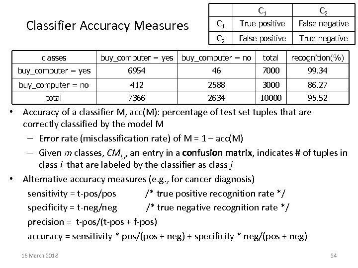C 1 Classifier Accuracy Measures C 2 C 1 True positive False negative C 2 False positive True negative classes buy_computer = yes buy_computer = no total recognition(%) buy_computer = yes 6954 46 7000 99. 34 buy_computer = no 412 2588 3000 86. 27 total 7366 2634 10000 95. 52 • Accuracy of a classifier M, acc(M): percentage of test set tuples that are correctly classified by the model M – Error rate (misclassification rate) of M = 1 – acc(M) – Given m classes, CMi, j, an entry in a confusion matrix, indicates # of tuples in class i that are labeled by the classifier as class j • Alternative accuracy measures (e. g. , for cancer diagnosis) sensitivity = t-pos/pos /* true positive recognition rate */ specificity = t-neg/neg /* true negative recognition rate */ precision = t-pos/(t-pos + f-pos) accuracy = sensitivity * pos/(pos + neg) + specificity * neg/(pos + neg) 16 March 2018 34

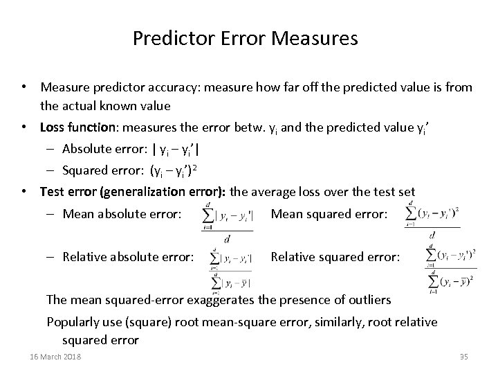Predictor Error Measures • Measure predictor accuracy: measure how far off the predicted value is from the actual known value • Loss function: measures the error betw. yi and the predicted value yi’ – Absolute error: | yi – yi’| – Squared error: (yi – yi’)2 • Test error (generalization error): the average loss over the test set – Mean absolute error: Mean squared error: – Relative absolute error: Relative squared error: The mean squared-error exaggerates the presence of outliers Popularly use (square) root mean-square error, similarly, root relative squared error 16 March 2018 35

Evaluating the Accuracy of a Classifier or Predictor (I) • Holdout method – Given data is randomly partitioned into two independent sets • Training set (e. g. , 2/3) for model construction • Test set (e. g. , 1/3) for accuracy estimation – Random sampling: a variation of holdout • Repeat holdout k times, accuracy = avg. of the accuracies obtained • Cross-validation (k-fold, where k = 10 is most popular) – Randomly partition the data into k mutually exclusive subsets, each approximately equal size – At i-th iteration, use Di as test set and others as training set – Leave-one-out: k folds where k = # of tuples, for small sized data – Stratified cross-validation: folds are stratified so that class dist. in each fold is approx. the same as that in the initial data 16 March 2018 36

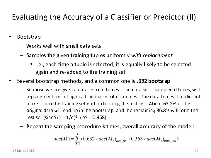Evaluating the Accuracy of a Classifier or Predictor (II) • Bootstrap – Works well with small data sets – Samples the given training tuples uniformly with replacement • i. e. , each time a tuple is selected, it is equally likely to be selected again and re-added to the training set • Several bootstrap methods, and a common one is. 632 bootsrap – Suppose we are given a data set of d tuples. The data set is sampled d times, with replacement, resulting in a training set of d samples. The data tuples that did not make it into the training set end up forming the test set. About 63. 2% of the original data will end up in the bootstrap, and the remaining 36. 8% will form the test set (since (1 – 1/d)d ≈ e-1 = 0. 368) – Repeat the sampling procedure k times, overall accuracy of the model: 16 March 2018 37

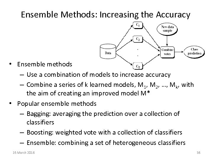Ensemble Methods: Increasing the Accuracy • Ensemble methods – Use a combination of models to increase accuracy – Combine a series of k learned models, M 1, M 2, …, Mk, with the aim of creating an improved model M* • Popular ensemble methods – Bagging: averaging the prediction over a collection of classifiers – Boosting: weighted vote with a collection of classifiers – Ensemble: combining a set of heterogeneous classifiers 16 March 2018 38

Clustering

What is Clustering? • Cluster: a collection of data objects – Similar to one another within the same cluster – Dissimilar to the objects in other clusters • Clustering/Cluster analysis – Finding similarities between data according to the characteristics found in the data and grouping similar data objects into clusters • Unsupervised learning: no predefined classes 16 March 2018 Clustering 40

Quality of Clustering • A good clustering method will produce high quality clusters with – high intra-class similarity – low inter-class similarity • The quality of a clustering result depends on both the similarity measure used by the method and its implementation • The quality of a clustering method is also measured by its ability to discover some or all of the hidden patterns 16 March 2018 Clustering 41

Measure the Quality of Clustering • Dissimilarity/Similarity metric: Similarity is expressed in terms of a distance function, typically metric: d(i, j) • The definitions of distance functions are usually very different for interval-scaled, boolean, categorical, ordinal, etc. variables. • Weights should be associated with different variables based on applications and data semantics. • It is hard to define “similar enough” or “good enough” – the answer is typically highly subjective. 16 March 2018 Clustering 42

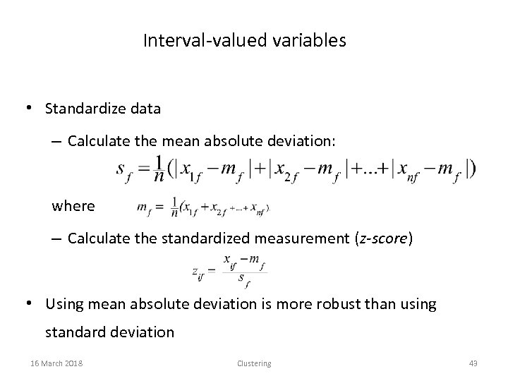Interval-valued variables • Standardize data – Calculate the mean absolute deviation: where – Calculate the standardized measurement (z-score) • Using mean absolute deviation is more robust than using standard deviation 16 March 2018 Clustering 43

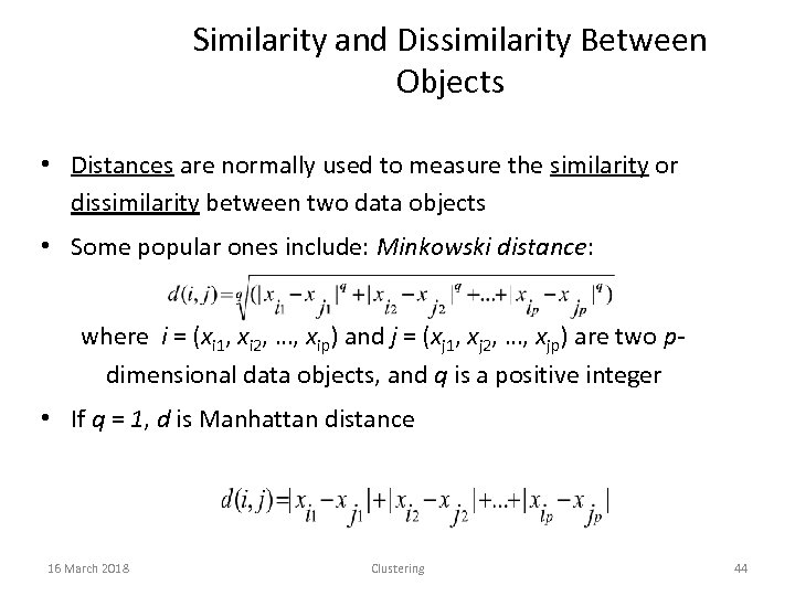Similarity and Dissimilarity Between Objects • Distances are normally used to measure the similarity or dissimilarity between two data objects • Some popular ones include: Minkowski distance: where i = (xi 1, xi 2, …, xip) and j = (xj 1, xj 2, …, xjp) are two pdimensional data objects, and q is a positive integer • If q = 1, d is Manhattan distance 16 March 2018 Clustering 44

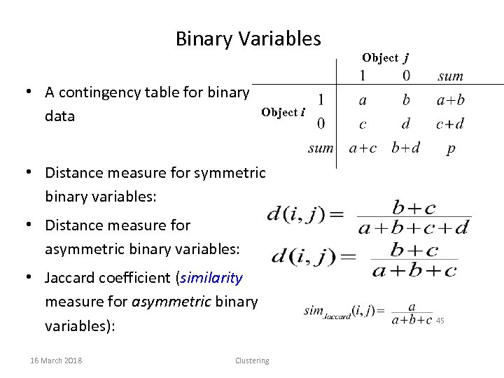Binary Variables • A contingency table for binary data Object j Object i • Distance measure for symmetric binary variables: • Distance measure for asymmetric binary variables: • Jaccard coefficient (similarity measure for asymmetric binary variables): 16 March 2018 Clustering 45

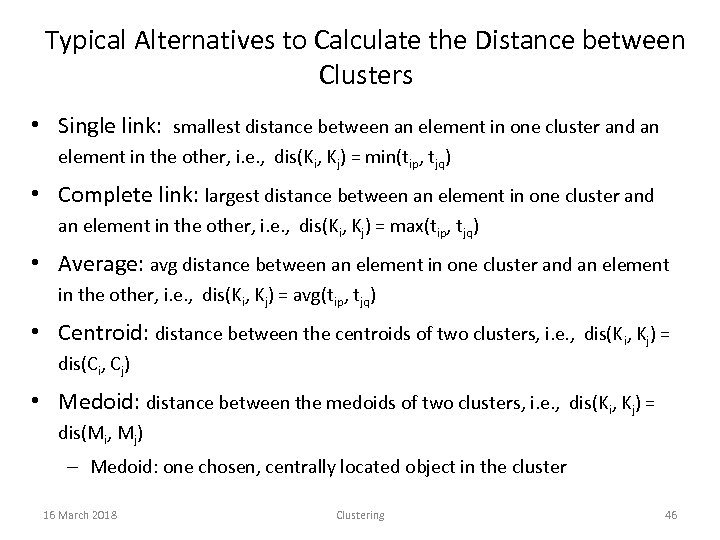Typical Alternatives to Calculate the Distance between Clusters • Single link: smallest distance between an element in one cluster and an element in the other, i. e. , dis(Ki, Kj) = min(tip, tjq) • Complete link: largest distance between an element in one cluster and an element in the other, i. e. , dis(Ki, Kj) = max(tip, tjq) • Average: avg distance between an element in one cluster and an element in the other, i. e. , dis(Ki, Kj) = avg(tip, tjq) • Centroid: distance between the centroids of two clusters, i. e. , dis(Ki, Kj) = dis(Ci, Cj) • Medoid: distance between the medoids of two clusters, i. e. , dis(Ki, Kj) = dis(Mi, Mj) – Medoid: one chosen, centrally located object in the cluster 16 March 2018 Clustering 46

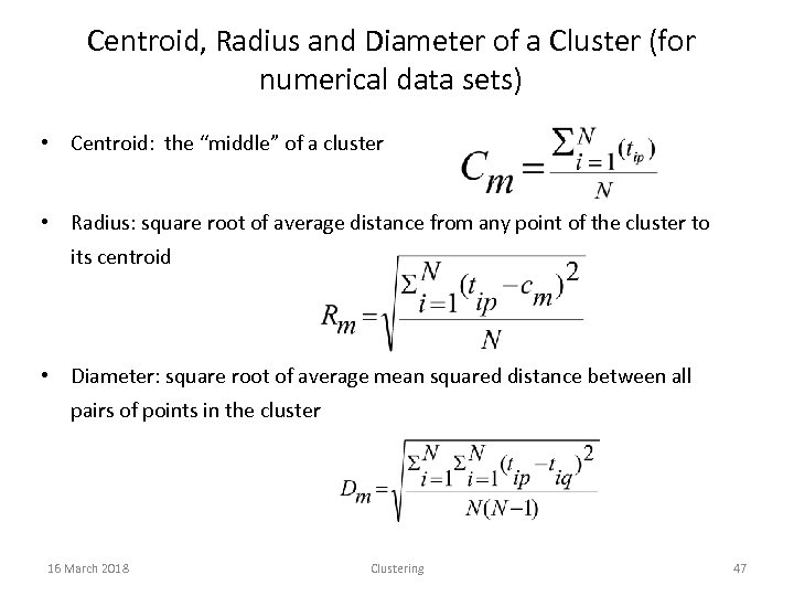Centroid, Radius and Diameter of a Cluster (for numerical data sets) • Centroid: the “middle” of a cluster • Radius: square root of average distance from any point of the cluster to its centroid • Diameter: square root of average mean squared distance between all pairs of points in the cluster 16 March 2018 Clustering 47

Major Clustering Approaches • Partitioning approach: – Construct various partitions and then evaluate them by some criterion, e. g. , minimizing the sum of squared distances – Typical methods: k-means, k-medoids, CLARANS • Hierarchical approach: – Create a hierarchical decomposition of the set of data (or objects) using some criterion – Typical methods: Diana, Agnes, BIRCH, ROCK, CAMELEON • Density-based approach: – Based on connectivity and density functions – Typical methods: DBSACN, OPTICS, Den. Clue 16 March 2018 Clustering 48

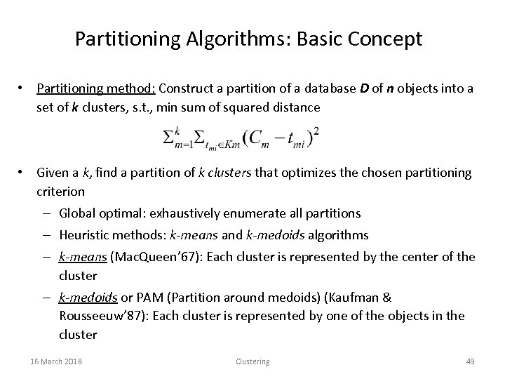Partitioning Algorithms: Basic Concept • Partitioning method: Construct a partition of a database D of n objects into a set of k clusters, s. t. , min sum of squared distance • Given a k, find a partition of k clusters that optimizes the chosen partitioning criterion – Global optimal: exhaustively enumerate all partitions – Heuristic methods: k-means and k-medoids algorithms – k-means (Mac. Queen’ 67): Each cluster is represented by the center of the cluster – k-medoids or PAM (Partition around medoids) (Kaufman & Rousseeuw’ 87): Each cluster is represented by one of the objects in the cluster 16 March 2018 Clustering 49

The K-Means Clustering Method • Given k, the k-means algorithm is implemented in four steps: – Partition objects into k nonempty subsets – Compute seed points as the centroids of the clusters of the current partition (the centroid is the center, i. e. , mean point, of the cluster) – Assign each object to the cluster with the nearest seed point – Go back to Step 2, stop when no more new assignment 16 March 2018 Clustering 50

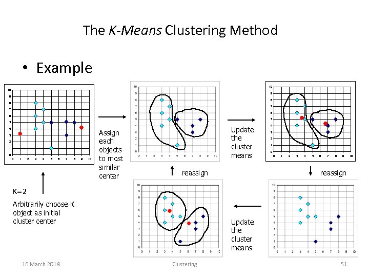The K-Means Clustering Method • Example 10 10 9 9 8 8 7 7 6 6 5 5 4 3 2 1 0 0 1 2 3 4 5 6 7 8 9 10 Assign each objects to most similar center Update the cluster means reassign 4 3 2 1 0 0 1 2 3 4 5 6 7 8 9 reassign K=2 Arbitrarily choose K object as initial cluster center 16 March 2018 Update the cluster means Clustering 51 10

The K-Medoids Clustering Method • Find representative objects, called medoids, in clusters • PAM (Partitioning Around Medoids, 1987) – starts from an initial set of medoids and iteratively replaces one of the medoids by one of the non-medoids if it improves the total distance of the resulting clustering – PAM works effectively for small data sets, but does not scale well for large data sets • CLARA (Kaufmann & Rousseeuw, 1990) • CLARANS (Ng & Han, 1994): Randomized sampling 16 March 2018 Clustering 52

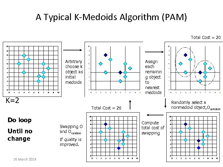A Typical K-Medoids Algorithm (PAM) Total Cost = 20 10 9 8 Arbitrary choose k object as initial medoids 7 6 5 4 3 2 Assign each remainin g object to nearest medoids 1 0 0 1 2 3 4 5 6 7 8 9 10 K=2 Randomly select a nonmedoid object, Oramdom Total Cost = 26 Do loop Until no change 10 10 9 Swapping O and Orandom Compute total cost of swapping 8 7 6 9 8 7 6 5 4 4 3 3 2 2 1 If quality is improved. 5 1 0 16 March 2018 0 0 1 2 3 4 5 Clustering 6 7 8 9 10 0 1 2 3 4 5 6 7 8 53 9 10

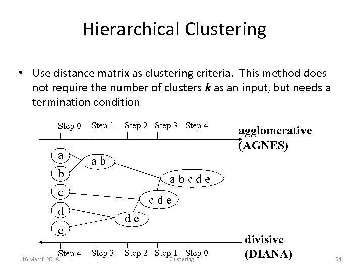Hierarchical Clustering • Use distance matrix as clustering criteria. This method does not require the number of clusters k as an input, but needs a termination condition Step 0 a b Step 1 Step 2 Step 3 Step 4 ab abcde c cde d de e Step 4 16 March 2018 agglomerative (AGNES) Step 3 Step 2 Step 1 Step 0 Clustering divisive (DIANA) 54

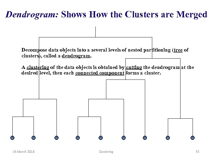Dendrogram: Shows How the Clusters are Merged Decompose data objects into a several levels of nested partitioning (tree of clusters), called a dendrogram. A clustering of the data objects is obtained by cutting the dendrogram at the desired level, then each connected component forms a cluster. 16 March 2018 Clustering 55

BIRCH (1996) • Birch: Balanced Iterative Reducing and Clustering using Hierarchies (Zhang, Ramakrishnan & Livny, SIGMOD’ 96) • Incrementally construct a CF (Clustering Feature) tree, a hierarchical data structure for multiphase clustering – Phase 1: scan DB to build an initial in-memory CF tree (a multi -level compression of the data that tries to preserve the inherent clustering structure of the data) – Phase 2: use an arbitrary clustering algorithm to cluster the leaf nodes of the CF-tree • Scales linearly: finds a good clustering with a single scan and improves the quality with a few additional scans • Weakness: handles only numeric data, and sensitive to the order of the data record. 16 March 2018 Clustering 56

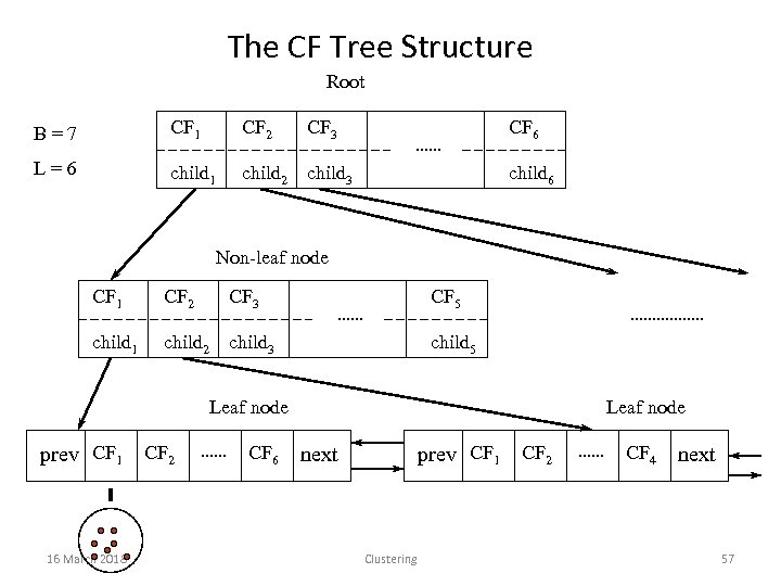The CF Tree Structure Root B=7 CF 1 CF 2 CF 3 CF 6 L=6 child 1 child 2 child 3 child 6 Non-leaf node CF 1 CF 2 CF 3 CF 5 child 1 child 2 child 3 child 5 Leaf node prev CF 1 16 March 2018 CF 2 CF 6 Leaf node prev CF 1 next Clustering CF 2 CF 4 next 57

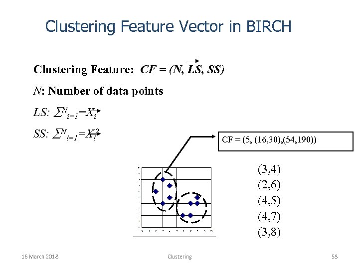Clustering Feature Vector in BIRCH Clustering Feature: CF = (N, LS, SS) N: Number of data points LS: Ni=1=Xi SS: Ni=1=Xi 2 CF = (5, (16, 30), (54, 190)) (3, 4) (2, 6) (4, 5) (4, 7) (3, 8) 16 March 2018 Clustering 58

Density-Based Clustering Methods • Clustering based on density (local cluster criterion), such as density-connected points • Major features: – Discover clusters of arbitrary shape – Handle noise – One scan – Need density parameters as termination condition • Well-known examples: – DBSCAN: Ester, et al. (KDD’ 96) – OPTICS: Ankerst, et al (SIGMOD’ 99). – DENCLUE: Hinneburg & D. Keim (KDD’ 98) – CLIQUE: Agrawal, et al. (SIGMOD’ 98) (more grid-based) 16 March 2018 Clustering 59

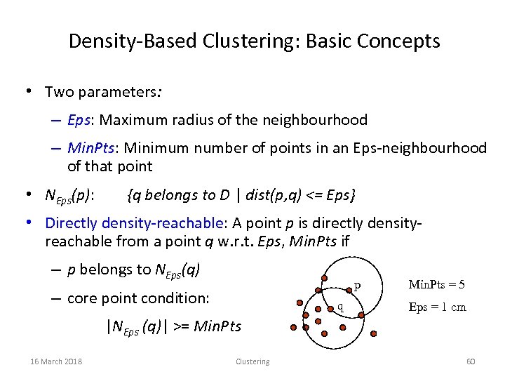Density-Based Clustering: Basic Concepts • Two parameters: – Eps: Maximum radius of the neighbourhood – Min. Pts: Minimum number of points in an Eps-neighbourhood of that point • NEps(p): {q belongs to D | dist(p, q) <= Eps} • Directly density-reachable: A point p is directly densityreachable from a point q w. r. t. Eps, Min. Pts if – p belongs to NEps(q) p – core point condition: q Min. Pts = 5 Eps = 1 cm |NEps (q)| >= Min. Pts 16 March 2018 Clustering 60

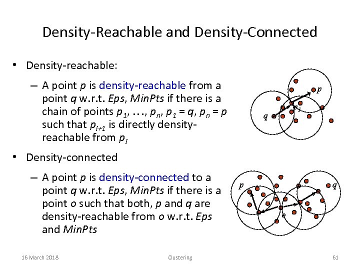Density-Reachable and Density-Connected • Density-reachable: – A point p is density-reachable from a point q w. r. t. Eps, Min. Pts if there is a chain of points p 1, …, pn, p 1 = q, pn = p such that pi+1 is directly densityreachable from pi p p 1 q • Density-connected – A point p is density-connected to a point q w. r. t. Eps, Min. Pts if there is a point o such that both, p and q are density-reachable from o w. r. t. Eps and Min. Pts 16 March 2018 Clustering p q o 61

Model-Based Clustering • What is model-based clustering? – Attempt to optimize the fit between the given data and some mathematical model – Based on the assumption: Data are generated by a mixture of underlying probability distribution • Typical methods – Statistical approach • EM (Expectation maximization), Auto. Class – Machine learning approach • COBWEB, CLASSIT – Neural network approach • SOM (Self-Organizing Feature Map) 16 March 2018 Clustering 62

What Is Outlier Discovery? • What are outliers? – The set of objects are considerably dissimilar from the remainder of the data – Example: ? ? ? • Problem: Define and find outliers in large data sets • Applications: – Credit card fraud detection – Telecom fraud detection – Customer segmentation – Medical analysis 16 March 2018 Clustering 63

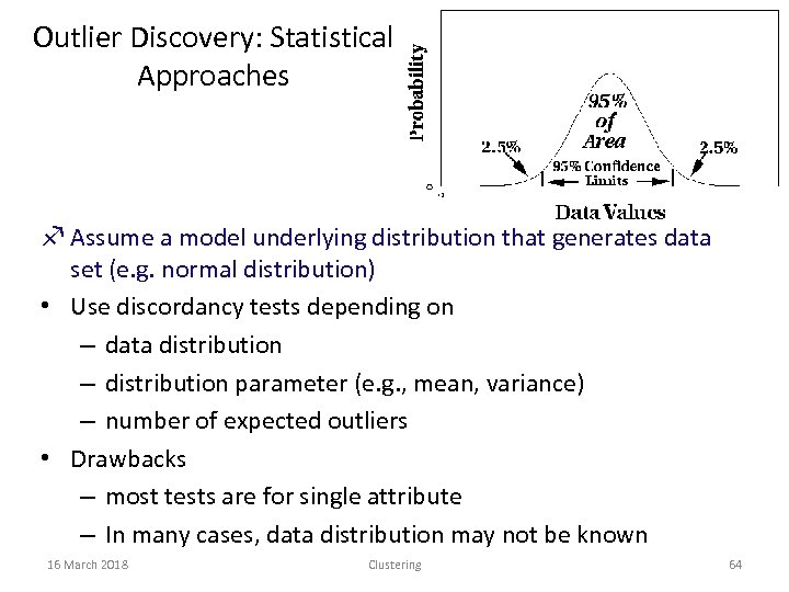Outlier Discovery: Statistical Approaches f Assume a model underlying distribution that generates data set (e. g. normal distribution) • Use discordancy tests depending on – data distribution – distribution parameter (e. g. , mean, variance) – number of expected outliers • Drawbacks – most tests are for single attribute – In many cases, data distribution may not be known 16 March 2018 Clustering 64

Outlier Discovery: Distance-Based Approach • Introduced to counter the main limitations imposed by statistical methods – We need multi-dimensional analysis without knowing data distribution • Distance-based outlier: A DB(p, D)-outlier is an object O in a dataset T such that at least a fraction p of the objects in T lies at a distance greater than D from O 16 March 2018 Clustering 65