OVERVIEW DATA MINING VESIT M VIJAYALAKSHMI Outline

OVERVIEW DATA MINING VESIT M. VIJAYALAKSHMI

Outline Of the Presentation – Motivation & Introduction – Data Mining Algorithms – Teaching Plan DATA MINING VESIT M. VIJAYALAKSHMI 2

Why Data Mining? Commercial Viewpoint • Lots of data is being collected and warehoused – Web data, e-commerce – purchases at department/grocery stores – Bank/Credit Card transactions • Computers have become cheaper and more powerful • Competitive Pressure is strong – Provide better, customized services for an edge (e. g. in Customer Relationship Management) DATA MINING VESIT M. VIJAYALAKSHMI 3

Typical Decision Making • Given a database of 100, 000 names, which persons are the least likely to default on their credit cards? • Which of my customers are likely to be the most loyal? • Which claims in insurance are potential frauds? • Who may not pay back loans? • Who are consistent players to bid for in IPL? • Who can be potential customers for a new toy? Data Mining helps extract such information DATA MINING VESIT M. VIJAYALAKSHMI 4

Why Mine Data? Scientific Viewpoint • Data collected and stored at enormous speeds (GB/hour) – remote sensors on a satellite – telescopes scanning the skies – microarrays generating gene expression data – scientific simulations generating terabytes of data • Traditional techniques infeasible for raw data • Data mining may help scientists – in classifying and segmenting data – in Hypothesis Formation DATA MINING VESIT M. VIJAYALAKSHMI 5

Mining Large Data Sets Motivation • There is often information “hidden” in the data that is not readily evident. • Human analysts may take weeks to discover useful information. DATA MINING VESIT M. VIJAYALAKSHMI 6

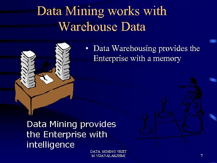Data Mining works with Warehouse Data • Data Warehousing provides the Enterprise with a memory z Data Mining provides the Enterprise with intelligence DATA MINING VESIT M. VIJAYALAKSHMI 7

What Is Data Mining? • Data mining (knowledge discovery in databases): – Extraction of interesting (non-trivial, implicit, previously unknown and potentially useful) information or patterns from data in large databases • Alternative names and their “inside stories”: – Knowledge discovery(mining) in databases (KDD), knowledge extraction, data/pattern analysis, data archeology, data dredging, information harvesting, business intelligence, etc. • What is not data mining? – (Deductive) query processing. – Expert systems or small ML/statistical programs DATA MINING VESIT M. VIJAYALAKSHMI 8

Potential Applications • Market analysis and management – target marketing, CRM, market basket analysis, cross selling, market segmentation • Risk analysis and management – Forecasting, customer retention, quality control, competitive analysis • Fraud detection and management • Text mining (news group, email, documents) and Web analysis. – Intelligent query answering DATA MINING VESIT M. VIJAYALAKSHMI 9

Other Applications • game statistics to gain competitive advantage Astronomy • JPL and the Palomar Observatory discovered 22 quasars with the help of data mining • IBM Surf-Aid applies data mining algorithms to Web access logs for market-related pages to discover customer preference and behavior pages, analyzing effectiveness of Web marketing, improving Web site organization, etc. DATA MINING VESIT M. VIJAYALAKSHMI 10

What makes data mining possible? • Advances in the following areas are making data mining deployable: – data warehousing – better and more data (i. e. , operational, behavioral, and demographic) – the emergence of easily deployed data mining tools and – the advent of new data mining techniques. – -- Gartner Group DATA MINING VESIT M. VIJAYALAKSHMI 11

What is Not Data Mining • Database – Find all credit applicants with last name of Smith. – Identify customers who have purchased more than $10, 000 in the last month. – Find all customers who have purchased milk • Data Mining – Find all credit applicants who are poor credit risks. (classification) – Identify customers with similar buying habits. (Clustering) – Find all items which are frequently purchased with milk. (association rules) DATA MINING VESIT M. VIJAYALAKSHMI 12

Data Mining: On What Kind of Data? • • Relational databases Data warehouses Transactional databases Advanced DB and information repositories – – – Object-oriented and object-relational databases Spatial databases Time-series data and temporal data Text databases and multimedia databases Heterogeneous and legacy databases WWW DATA MINING VESIT M. VIJAYALAKSHMI 13

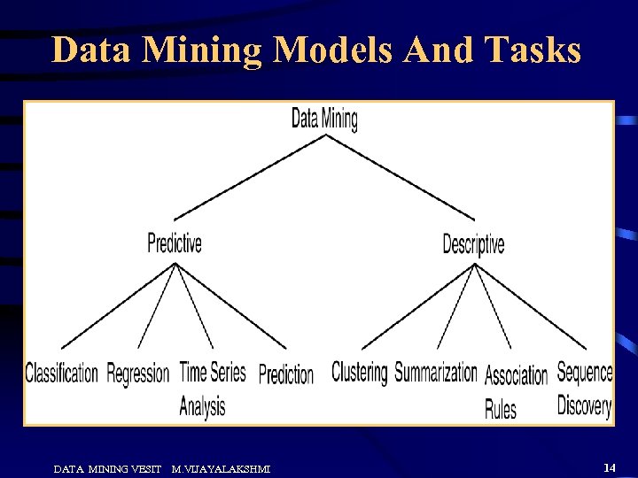Data Mining Models And Tasks DATA MINING VESIT M. VIJAYALAKSHMI 14

Are All the “Discovered” Patterns Interesting? • A data mining system/query may generate thousands of patterns, not all of them are interesting. • Interestingness measures: – A pattern is interesting if it is easily understood by humans, valid on new or test data with some degree of certainty, potentially useful, novel, or validates some hypothesis that a user seeks to confirm • Objective vs. subjective interestingness measures: – Objective: based on statistics and structures of patterns, e. g. , support, confidence, etc. – Subjective: based on user’s belief in the data, e. g. , unexpectedness, novelty, etc. DATA MINING VESIT M. VIJAYALAKSHMI 15

Can We Find All and Only Interesting Patterns? • Find all the interesting patterns: Completeness – Association vs. classification vs. clustering • Search for only interesting patterns: • First general all the patterns and then filter out the uninteresting ones. • Generate only the interesting paterns DATA MINING VESIT M. VIJAYALAKSHMI 16

Data Mining vs. KDD • Knowledge Discovery in Databases (KDD): process of finding useful information and patterns in data. • Data Mining: Use of algorithms to extract the information and patterns derived by the KDD process. DATA MINING VESIT M. VIJAYALAKSHMI 17

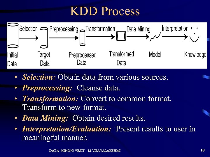KDD Process • Selection: Obtain data from various sources. • Preprocessing: Cleanse data. • Transformation: Convert to common format. Transform to new format. • Data Mining: Obtain desired results. • Interpretation/Evaluation: Present results to user in meaningful manner. DATA MINING VESIT M. VIJAYALAKSHMI 18

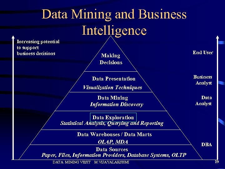Data Mining and Business Intelligence Increasing potential to support business decisions Making Decisions Data Presentation Visualization Techniques Data Mining Information Discovery End User Business Analyst Data Exploration Statistical Analysis, Querying and Reporting Data Warehouses / Data Marts OLAP, MDA Data Sources Paper, Files, Information Providers, Database Systems, OLTP DATA MINING VESIT M. VIJAYALAKSHMI DBA 19

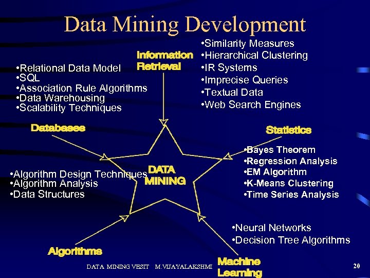Data Mining Development • Relational Data Model • SQL • Association Rule Algorithms • Data Warehousing • Scalability Techniques • Similarity Measures • Hierarchical Clustering • IR Systems • Imprecise Queries • Textual Data • Web Search Engines • Bayes Theorem • Regression Analysis • EM Algorithm • K-Means Clustering • Time Series Analysis • Algorithm Design Techniques • Algorithm Analysis • Data Structures • Neural Networks • Decision Tree Algorithms DATA MINING VESIT M. VIJAYALAKSHMI 20

Data Mining Issues • • Human Interaction Overfitting Outliers Interpretation Visualization Large Datasets High Dimensionality DATA MINING VESIT M. VIJAYALAKSHMI • • Multimedia Data Missing Data Irrelevant Data Noisy Data Changing Data Integration Application 21

Social Implications of DM • Privacy • Profiling • Unauthorized use DATA MINING VESIT M. VIJAYALAKSHMI 22

Data Mining Metrics • • Usefulness Return on Investment (ROI) Accuracy Space/Time DATA MINING VESIT M. VIJAYALAKSHMI 23

Data Mining Algorithms 1. Classification 2. Clustering 3. Association Mining 4. Web Mining DATA MINING VESIT M. VIJAYALAKSHMI

Data Mining Tasks • Prediction Methods – Use some variables to predict unknown or future values of other variables. • Description Methods – Find human-interpretable patterns that describe the data. DATA MINING VESIT M. VIJAYALAKSHMI 25

Data Mining Algorithms • • • Classification [Predictive] Clustering [Descriptive] Association Rule Discovery [Descriptive] Sequential Pattern Discovery [Descriptive] Regression [Predictive] Deviation Detection [Predictive] DATA MINING VESIT M. VIJAYALAKSHMI 26

Data Mining Algorithms CLASSIFICATION DATA MINING VESIT M. VIJAYALAKSHMI

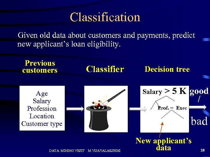Classification Given old data about customers and payments, predict new applicant’s loan eligibility. Previous customers Classifier Salary Age Salary Profession Location Customer type DATA MINING VESIT Decision tree > 5 K good / Prof. = Exec bad M. VIJAYALAKSHMI New applicant’s data 28

Classification Problem • Given a database D={t 1, t 2, …, tn} and a set of classes C={C 1, …, Cm}, the Classification Problem is to define a mapping f: Dg. C where each ti is assigned to one class. • Actually divides D into equivalence classes. • Prediction is similar, but may be viewed as having infinite number of classes. DATA MINING VESIT M. VIJAYALAKSHMI 29

Supervised vs. Unsupervised Learning • Supervised learning (classification) – Supervision: The training data (observations, measurements, etc. ) are accompanied by labels indicating the class of the observations – New data is classified based on the training set • Unsupervised learning (clustering) – The class labels of training data is unknown – Given a set of measurements, observations, etc. with the aim of establishing the existence of classes or clusters in the data DATA MINING VESIT M. VIJAYALAKSHMI 30

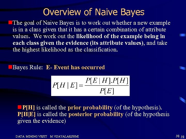Overview of Naive Bayes n. The goal of Naive Bayes is to work out whether a new example is in a class given that it has a certain combination of attribute values. We work out the likelihood of the example being in each class given the evidence (its attribute values), and take the highest likelihood as the classification. n. Bayes Rule: E- Event has occurred n. P[H] is called the prior probability (of the hypothesis). P[H|E] is called the posterior probability (of the hypothesis given the evidence) DATA MINING VESIT M. VIJAYALAKSHMI 31 31

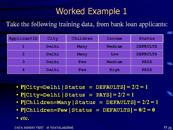Worked Example 1 Take the following training data, from bank loan applicants: Applicant. ID City Children Income Status 1 Delhi Many Medium DEFAULTS 2 Delhi Many Low DEFAULTS 3 Delhi Few Medium PAYS 4 Delhi Few High PAYS • • • P[City=Delhi | Status = DEFAULTS] = 2/2 = 1 P[City=Delhi | Status = PAYS] = 2/2 = 1 P[Children=Many | Status = DEFAULTS] = 2/2 = 1 P[Children=Few | Status = DEFAULTS] = 0/2 = 0 etc. DATA MINING VESIT M. VIJAYALAKSHMI 32 32

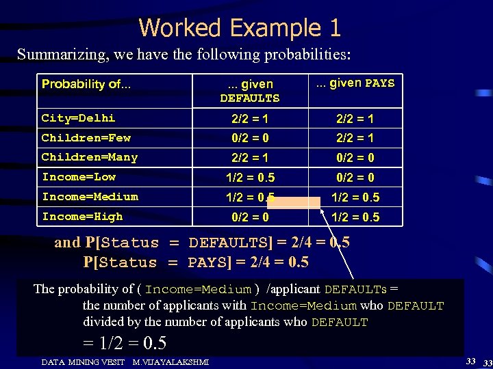Worked Example 1 Summarizing, we have the following probabilities: . . . given DEFAULTS . . . given PAYS City=Delhi 2/2 = 1 Children=Few 0/2 = 0 2/2 = 1 Children=Many 2/2 = 1 0/2 = 0 Income=Low 1/2 = 0. 5 0/2 = 0 Income=Medium 1/2 = 0. 5 0/2 = 0 1/2 = 0. 5 Probability of. . . Income=High and P[Status = DEFAULTS] = 2/4 = 0. 5 P[Status = PAYS] = 2/4 = 0. 5 The probability of ( Income=Medium ) /applicant DEFAULTs = the number of applicants with Income=Medium who DEFAULT divided by the number of applicants who DEFAULT = 1/2 = 0. 5 DATA MINING VESIT M. VIJAYALAKSHMI 33 33

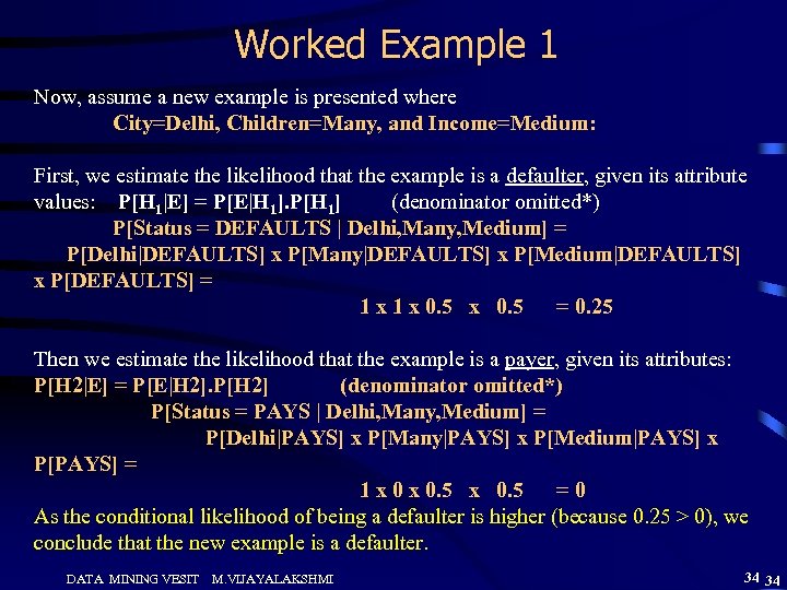Worked Example 1 Now, assume a new example is presented where City=Delhi, Children=Many, and Income=Medium: First, we estimate the likelihood that the example is a defaulter, given its attribute values: P[H 1|E] = P[E|H 1]. P[H 1] (denominator omitted*) P[Status = DEFAULTS | Delhi, Many, Medium] = P[Delhi|DEFAULTS] x P[Many|DEFAULTS] x P[Medium|DEFAULTS] x P[DEFAULTS] = 1 x 0. 5 = 0. 25 Then we estimate the likelihood that the example is a payer, given its attributes: P[H 2|E] = P[E|H 2]. P[H 2] (denominator omitted*) P[Status = PAYS | Delhi, Many, Medium] = P[Delhi|PAYS] x P[Many|PAYS] x P[Medium|PAYS] x P[PAYS] = 1 x 0. 5 =0 As the conditional likelihood of being a defaulter is higher (because 0. 25 > 0), we conclude that the new example is a defaulter. DATA MINING VESIT M. VIJAYALAKSHMI 34 34

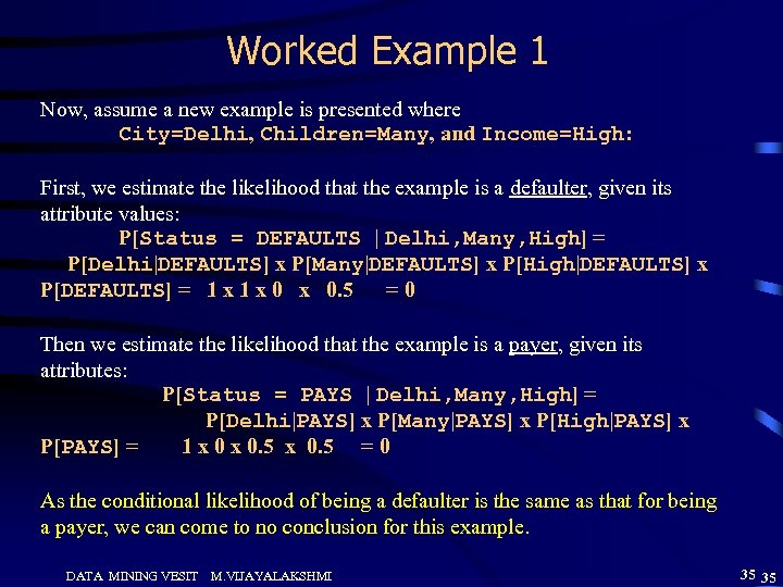Worked Example 1 Now, assume a new example is presented where City=Delhi, Children=Many, and Income=High: First, we estimate the likelihood that the example is a defaulter, given its attribute values: P[Status = DEFAULTS | Delhi, Many, High] = P[Delhi|DEFAULTS] x P[Many|DEFAULTS] x P[High|DEFAULTS] x P[DEFAULTS] = 1 x 0 x 0. 5 =0 Then we estimate the likelihood that the example is a payer, given its attributes: P[Status = PAYS | Delhi, Many, High] = P[Delhi|PAYS] x P[Many|PAYS] x P[High|PAYS] x P[PAYS] = 1 x 0. 5 = 0 As the conditional likelihood of being a defaulter is the same as that for being a payer, we can come to no conclusion for this example. DATA MINING VESIT M. VIJAYALAKSHMI 35 35

Weaknesses • Naive Bayes assumes that variables are equally important and that they are independent which is often not the case in practice. • Naive Bayes is damaged by the inclusion of redundant (strongly dependent) attributes. • Sparse data: If some attribute values are not present in the data, then a zero probability for P[E|H] might exist. This would lead P[H|E] to be zero no matter how high P[E|H] is for other attribute values. Small positive values which estimate the so-called ‘prior probabilities’ are often used to correct this. DATA MINING VESIT M. VIJAYALAKSHMI 36 36

Classification Using Decision Trees • Partitioning based: Divide search space into rectangular regions. • Tuple placed into class based on the region within which it falls. • DT approaches differ in how the tree is built: DT Induction • Internal nodes associated with attribute and arcs with values for that attribute. • Algorithms: ID 3, C 4. 5, CART DATA MINING VESIT M. VIJAYALAKSHMI 37

DT Issues • • Choosing Splitting Attributes Ordering of Splitting Attributes Splits Tree Structure Stopping Criteria Training Data Pruning DATA MINING VESIT M. VIJAYALAKSHMI 38

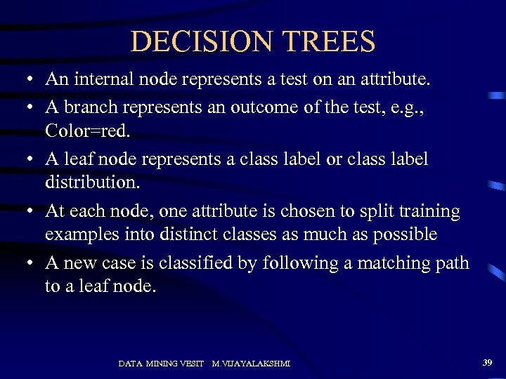DECISION TREES • An internal node represents a test on an attribute. • A branch represents an outcome of the test, e. g. , Color=red. • A leaf node represents a class label or class label distribution. • At each node, one attribute is chosen to split training examples into distinct classes as much as possible • A new case is classified by following a matching path to a leaf node. DATA MINING VESIT M. VIJAYALAKSHMI 39

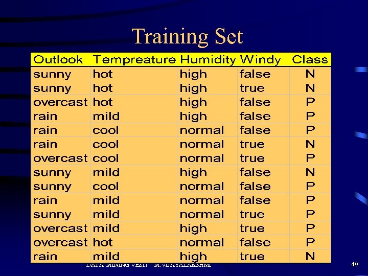Training Set DATA MINING VESIT M. VIJAYALAKSHMI 40

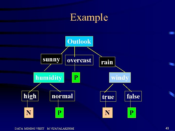Example Outlook sunny overcast humidity high N DATA MINING VESIT rain windy P normal P M. VIJAYALAKSHMI true false N P 41

Building Decision Tree • Top-down tree construction – At start, all training examples are at the root. – Partition the examples recursively by choosing one attribute each time. • Bottom-up tree pruning – Remove subtrees or branches, in a bottom-up manner, to improve the estimated accuracy on new cases. • Use of decision tree: Classifying an unknown sample – Test the attribute values of the sample against the decision tree DATA MINING VESIT M. VIJAYALAKSHMI 42

Algorithm for Decision Tree Induction • Basic algorithm (a greedy algorithm) – Tree is constructed in a top-down recursive divide-andconquer manner – At start, all the training examples are at the root – Attributes are categorical – Examples are partitioned recursively based on selected attributes – Test attributes are selected on the basis of a heuristic or statistical measure (e. g. , information gain) • Conditions for stopping partitioning – All samples for a given node belong to the same class – There are no remaining attributes for further partitioning – majority voting is employed for classifying the leaf – There are no samples left DATA MINING VESIT M. VIJAYALAKSHMI 43

Choosing the Splitting Attribute • At each node, available attributes are evaluated on the basis of separating the classes of the training examples. A Goodness function is used for this purpose. • Typical goodness functions: – information gain (ID 3/C 4. 5) – information gain ratio – gini index DATA MINING VESIT M. VIJAYALAKSHMI 44

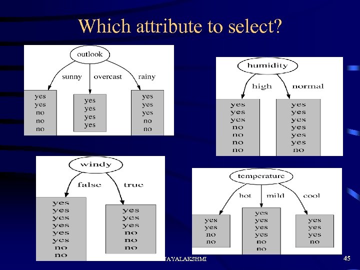Which attribute to select? DATA MINING VESIT M. VIJAYALAKSHMI 45

A criterion for attribute selection • Which is the best attribute? – The one which will result in the smallest tree – Heuristic: choose the attribute that produces the “purest” nodes • Popular impurity criterion: information gain – Information gain increases with the average purity of the subsets that an attribute produces • Strategy: choose attribute that results in greatest information gain DATA MINING VESIT M. VIJAYALAKSHMI 46

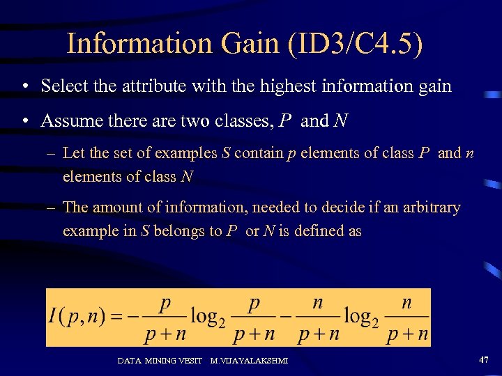Information Gain (ID 3/C 4. 5) • Select the attribute with the highest information gain • Assume there are two classes, P and N – Let the set of examples S contain p elements of class P and n elements of class N – The amount of information, needed to decide if an arbitrary example in S belongs to P or N is defined as DATA MINING VESIT M. VIJAYALAKSHMI 47

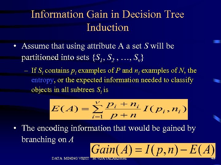Information Gain in Decision Tree Induction • Assume that using attribute A a set S will be partitioned into sets {S 1, S 2 , …, Sv} – If Si contains pi examples of P and ni examples of N, the entropy, or the expected information needed to classify objects in all subtrees Si is • The encoding information that would be gained by branching on A DATA MINING VESIT M. VIJAYALAKSHMI 48

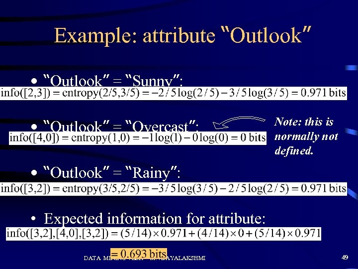Example: attribute “Outlook” • “Outlook” = “Sunny”: • “Outlook” = “Overcast”: Note: this is normally not defined. • “Outlook” = “Rainy”: • Expected information for attribute: DATA MINING VESIT M. VIJAYALAKSHMI 49

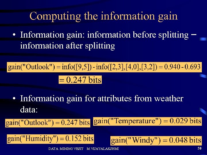Computing the information gain • Information gain: information before splitting – information after splitting • Information gain for attributes from weather data: DATA MINING VESIT M. VIJAYALAKSHMI 50

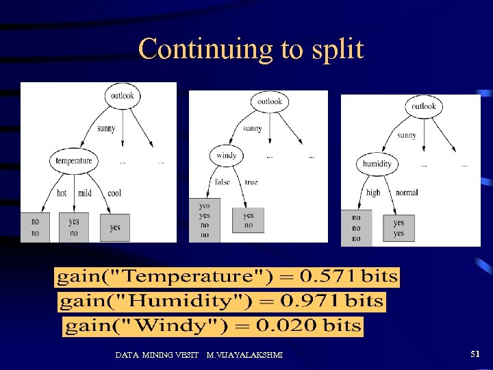Continuing to split DATA MINING VESIT M. VIJAYALAKSHMI 51

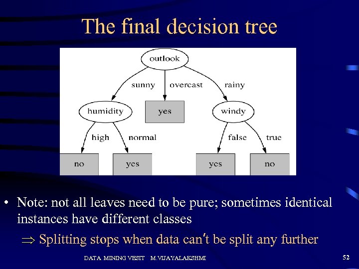The final decision tree • Note: not all leaves need to be pure; sometimes identical instances have different classes Splitting stops when data can’t be split any further DATA MINING VESIT M. VIJAYALAKSHMI 52

Avoid Overfitting in Classification • The generated tree may overfit the training data – Too many branches, some may reflect anomalies due to noise or outliers – Result is in poor accuracy for unseen samples • Two approaches to avoid overfitting – Prepruning: Halt tree construction early—do not split a node if this would result in the goodness measure falling below a threshold • Difficult to choose an appropriate threshold – Postpruning: Remove branches from a “fully grown” tree —get a sequence of progressively pruned trees • Use a set of data different from the training data to decide which is the “best pruned tree” DATA MINING VESIT M. VIJAYALAKSHMI 53

Data Mining Algorithms Clustering

Examples of Clustering Applications • Marketing: Help marketers discover distinct groups in their customer bases, and then use this knowledge to develop targeted marketing programs • Land use: Identification of areas of similar land use in an earth observation database • Insurance: Identifying groups of motor insurance policy holders with a high average claim cost • City-planning: Identifying groups of houses according to their house type, value, and geographical location • Earth-quake studies: Observed earth quake epicenters should be clustered along continent faults DATA MINING VESIT M. VIJAYALAKSHMI 56

Clustering vs. Classification • No prior knowledge – Number of clusters – Meaning of clusters – Cluster results are dynamic • Unsupervised learning DATA MINING VESIT M. VIJAYALAKSHMI 57

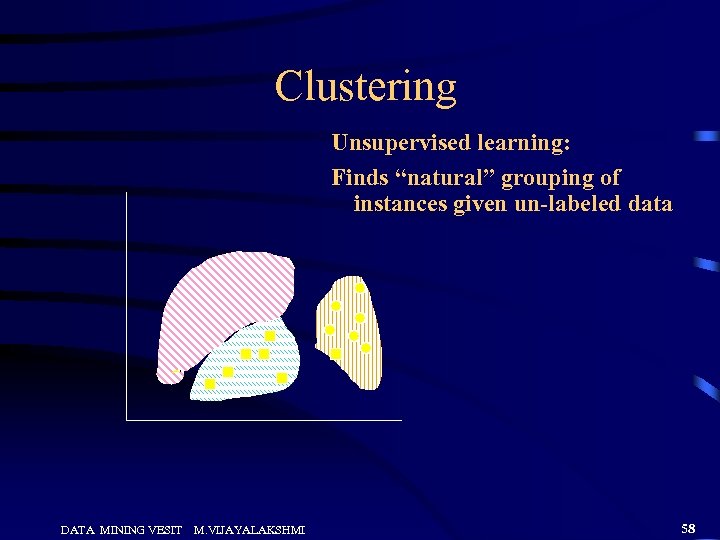Clustering Unsupervised learning: Finds “natural” grouping of instances given un-labeled data DATA MINING VESIT M. VIJAYALAKSHMI 58

Clustering Methods • Many different method and algorithms: – For numeric and/or symbolic data – Deterministic vs. probabilistic – Exclusive vs. overlapping – Hierarchical vs. flat – Top-down vs. bottom-up DATA MINING VESIT M. VIJAYALAKSHMI 59

Clustering Issues • • Outlier handling Dynamic data Interpreting results Evaluating results Number of clusters Data to be used Scalability DATA MINING VESIT M. VIJAYALAKSHMI 60

Clustering Evaluation • Manual inspection • Benchmarking on existing labels • Cluster quality measures – distance measures – high similarity within a cluster, low across clusters DATA MINING VESIT M. VIJAYALAKSHMI 61

Measure the Quality of Clustering • Dissimilarity/Similarity metric: Similarity is expressed in terms of a distance function, which is typically metric: d(i, j) • There is a separate “quality” function that measures the “goodness” of a cluster. • The definitions of distance functions are usually very different for interval-scaled, boolean, categorical, ordinal and ratio variables. • Weights should be associated with different variables based on applications and data semantics. • It is hard to define “similar enough” or “good enough” – the answer is typically highly subjective. DATA MINING VESIT M. VIJAYALAKSHMI 62

Type of data in clustering analysis • Interval-scaled variables: • Binary variables: • Nominal, ordinal, and ratio variables: • Variables of mixed types: DATA MINING VESIT M. VIJAYALAKSHMI 63

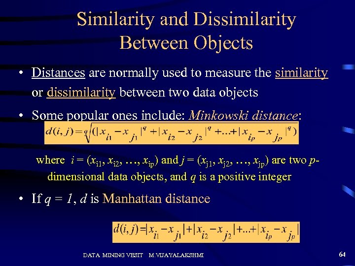Similarity and Dissimilarity Between Objects • Distances are normally used to measure the similarity or dissimilarity between two data objects • Some popular ones include: Minkowski distance: where i = (xi 1, xi 2, …, xip) and j = (xj 1, xj 2, …, xjp) are two pdimensional data objects, and q is a positive integer • If q = 1, d is Manhattan distance DATA MINING VESIT M. VIJAYALAKSHMI 64

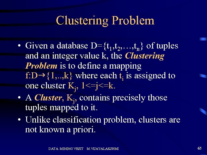Clustering Problem • Given a database D={t 1, t 2, …, tn} of tuples and an integer value k, the Clustering Problem is to define a mapping f: Dg{1, . . , k} where each ti is assigned to one cluster Kj, 1<=j<=k. • A Cluster, Kj, contains precisely those tuples mapped to it. • Unlike classification problem, clusters are not known a priori. DATA MINING VESIT M. VIJAYALAKSHMI 65

Types of Clustering • Hierarchical – Nested set of clusters created. • Partitional – One set of clusters created. • Incremental – Each element handled one at a time. • Simultaneous – All elements handled together. • Overlapping/Non-overlapping DATA MINING VESIT M. VIJAYALAKSHMI 66

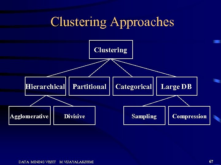Clustering Approaches Clustering Hierarchical Agglomerative DATA MINING VESIT Partitional Divisive M. VIJAYALAKSHMI Categorical Sampling Large DB Compression 67

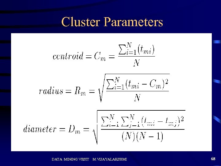Cluster Parameters DATA MINING VESIT M. VIJAYALAKSHMI 68

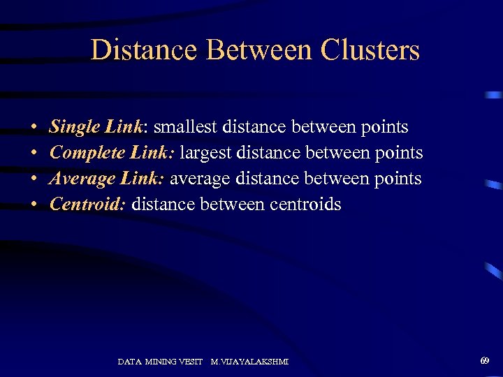Distance Between Clusters • • Single Link: smallest distance between points Complete Link: largest distance between points Average Link: average distance between points Centroid: distance between centroids DATA MINING VESIT M. VIJAYALAKSHMI 69

Hierarchical Clustering • Clusters are created in levels actually creating sets of clusters at each level. • Agglomerative – Initially each item in its own cluster – Iteratively clusters are merged together – Bottom Up • Divisive – Initially all items in one cluster – Large clusters are successively divided – Top Down DATA MINING VESIT M. VIJAYALAKSHMI 70

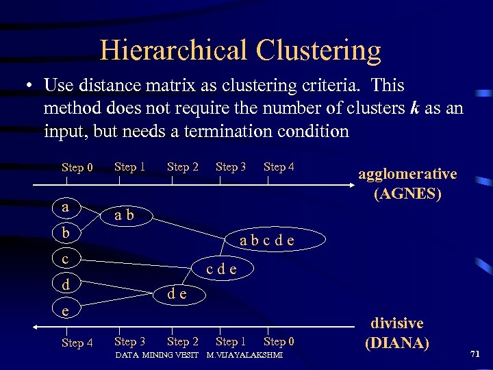Hierarchical Clustering • Use distance matrix as clustering criteria. This method does not require the number of clusters k as an input, but needs a termination condition Step 0 a b Step 1 Step 2 Step 4 agglomerative (AGNES) ab abcde c cde d de e Step 4 Step 3 Step 2 DATA MINING VESIT Step 1 Step 0 M. VIJAYALAKSHMI divisive (DIANA) 71

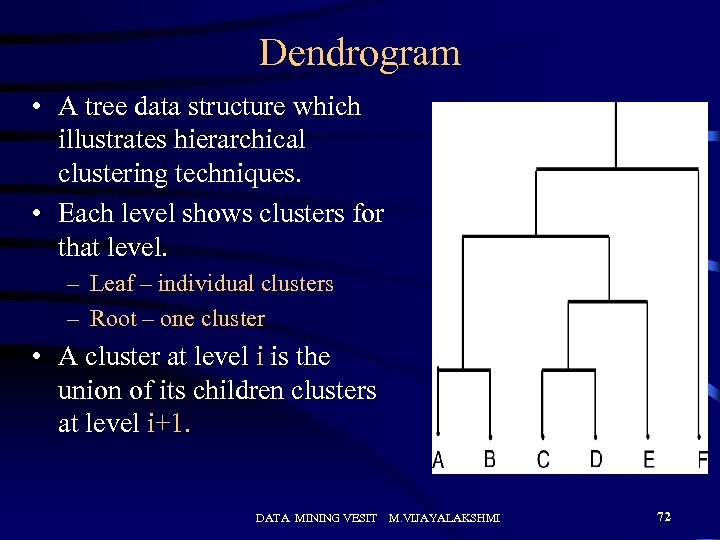Dendrogram • A tree data structure which illustrates hierarchical clustering techniques. • Each level shows clusters for that level. – Leaf – individual clusters – Root – one cluster • A cluster at level i is the union of its children clusters at level i+1. DATA MINING VESIT M. VIJAYALAKSHMI 72

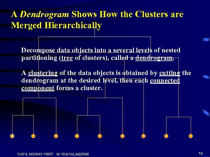A Dendrogram Shows How the Clusters are Merged Hierarchically Decompose data objects into a several levels of nested partitioning (tree of clusters), called a dendrogram. A clustering of the data objects is obtained by cutting the dendrogram at the desired level, then each connected component forms a cluster. DATA MINING VESIT M. VIJAYALAKSHMI 73

DIANA (Divisive Analysis) • Implemented in statistical analysis packages, e. g. , Splus • Inverse order of AGNES • Eventually each node forms a cluster on its own DATA MINING VESIT M. VIJAYALAKSHMI 74

Partitional Clustering • Nonhierarchical • Creates clusters in one step as opposed to several steps. • Since only one set of clusters is output, the user normally has to input the desired number of clusters, k. • Usually deals with static sets. DATA MINING VESIT M. VIJAYALAKSHMI 75

K-Means • Initial set of clusters randomly chosen. • Iteratively, items are moved among sets of clusters until the desired set is reached. • High degree of similarity among elements in a cluster is obtained. • Given a cluster Ki={ti 1, ti 2, …, tim}, the cluster mean is mi = (1/m)(ti 1 + … + tim) DATA MINING VESIT M. VIJAYALAKSHMI 76

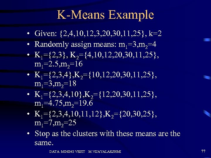K-Means Example • Given: {2, 4, 10, 12, 3, 20, 30, 11, 25}, k=2 • Randomly assign means: m 1=3, m 2=4 • K 1={2, 3}, K 2={4, 10, 12, 20, 30, 11, 25}, m 1=2. 5, m 2=16 • K 1={2, 3, 4}, K 2={10, 12, 20, 30, 11, 25}, m 1=3, m 2=18 • K 1={2, 3, 4, 10}, K 2={12, 20, 30, 11, 25}, m 1=4. 75, m 2=19. 6 • K 1={2, 3, 4, 10, 11, 12}, K 2={20, 30, 25}, m 1=7, m 2=25 • Stop as the clusters with these means are the same. DATA MINING VESIT M. VIJAYALAKSHMI 77

The K-Means Clustering Method • Given k, the k-means algorithm is implemented in 4 steps: – Partition objects into k nonempty subsets – Compute seed points as the centroids of the clusters of the current partition. The centroid is the center (mean point) of the cluster. – Assign each object to the cluster with the nearest seed point. – Go back to Step 2, stop when no more new assignment. DATA MINING VESIT M. VIJAYALAKSHMI 78

Comments on the K-Means Method • Strength – Relatively efficient: O(tkn), where n is # objects, k is # clusters, and t is # iterations. Normally, k, t << n. – Often terminates at a local optimum. The global optimum may be found using techniques such as: deterministic annealing and genetic algorithms • Weakness – Applicable only when mean is defined, then what about categorical data? – Need to specify k, the number of clusters, in advance – Unable to handle noisy data and outliers – Not suitable to discover clusters with non-convex shapes DATA MINING VESIT M. VIJAYALAKSHMI 79

The K-Medoids Clustering Method • Find representative objects, called medoids, in clusters • PAM (Partitioning Around Medoids, ) – starts from an initial set of medoids and iteratively replaces one of the medoids by one of the non-medoids if it improves the total distance of the resulting clustering – Handles outliers well. – Ordering of input does not impact results. – Does not scale well. – Each cluster represented by one item, called the medoid. – Initial set of k medoids randomly chosen. • PAM works effectively for small data sets, but does not scale well for large data sets DATA MINING VESIT M. VIJAYALAKSHMI 80

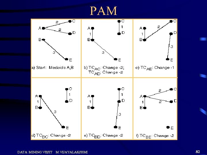
PAM (Partitioning Around Medoids) • PAM - Use real object to represent the cluster – Select k representative objects arbitrarily – For each pair of non-selected object h and selected object i, calculate the total swapping cost TCih – For each pair of i and h, • If TCih < 0, i is replaced by h • Then assign each non-selected object to the most similar representative object – repeat steps 2 -3 until there is no change DATA MINING VESIT M. VIJAYALAKSHMI 81

PAM DATA MINING VESIT M. VIJAYALAKSHMI 82

DATA MINING ASSOCIATION RULES

Example: Market Basket Data • Items frequently purchased together: Computer Printer • Uses: – Placement – Advertising – Sales – Coupons • Objective: increase sales and reduce costs • Called Market Basket Analysis, Shopping Cart Analysis DATA MINING VESIT M. VIJAYALAKSHMI 84

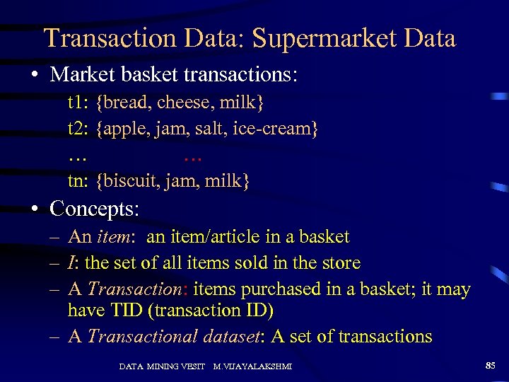Transaction Data: Supermarket Data • Market basket transactions: t 1: {bread, cheese, milk} t 2: {apple, jam, salt, ice-cream} … … tn: {biscuit, jam, milk} • Concepts: – An item: an item/article in a basket – I: the set of all items sold in the store – A Transaction: items purchased in a basket; it may have TID (transaction ID) – A Transactional dataset: A set of transactions DATA MINING VESIT M. VIJAYALAKSHMI 85

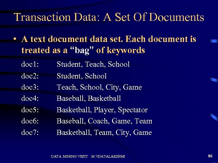Transaction Data: A Set Of Documents • A text document data set. Each document is treated as a “bag” of keywords doc 1: doc 2: doc 3: doc 4: doc 5: doc 6: doc 7: Student, Teach, School Student, School Teach, School, City, Game Baseball, Basketball, Player, Spectator Baseball, Coach, Game, Team Basketball, Team, City, Game DATA MINING VESIT M. VIJAYALAKSHMI 86

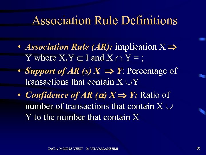Association Rule Definitions • Association Rule (AR): implication X Y where X, Y I and X Y = ; • Support of AR (s) X Y: Percentage of transactions that contain X Y • Confidence of AR (a) X Y: Ratio of number of transactions that contain X Y to the number that contain X DATA MINING VESIT M. VIJAYALAKSHMI 87

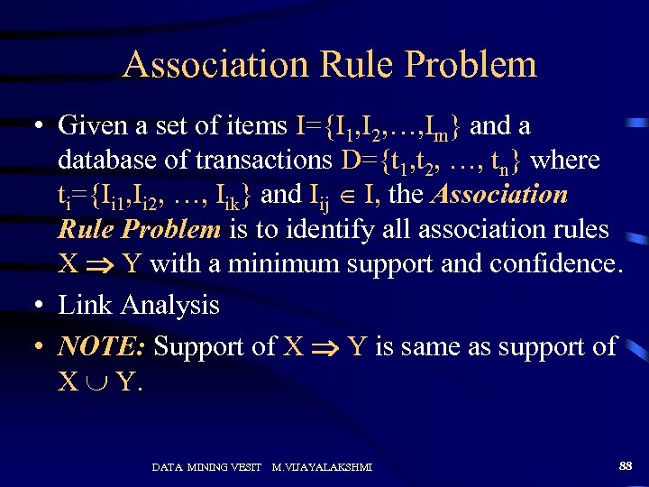Association Rule Problem • Given a set of items I={I 1, I 2, …, Im} and a database of transactions D={t 1, t 2, …, tn} where ti={Ii 1, Ii 2, …, Iik} and Iij I, the Association Rule Problem is to identify all association rules X Y with a minimum support and confidence. • Link Analysis • NOTE: Support of X Y is same as support of X Y. DATA MINING VESIT M. VIJAYALAKSHMI 88

Association Rule Mining Task • Given a set of transactions T, the goal of association rule mining is to find all rules having – support ≥ minsup threshold – confidence ≥ minconf threshold • Brute-force approach: – List all possible association rules – Compute the support and confidence for each rule – Prune rules that fail the minsup and minconf thresholds Computationally prohibitive! DATA MINING VESIT M. VIJAYALAKSHMI 89

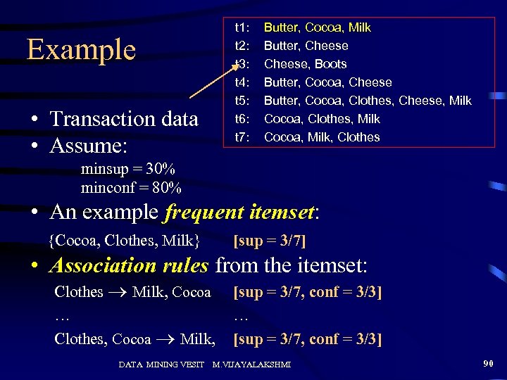t 1: t 2: t 3: t 4: t 5: t 6: t 7: Example • Transaction data • Assume: Butter, Cocoa, Milk Butter, Cheese, Boots Butter, Cocoa, Cheese Butter, Cocoa, Clothes, Cheese, Milk Cocoa, Clothes, Milk Cocoa, Milk, Clothes minsup = 30% minconf = 80% • An example frequent itemset: {Cocoa, Clothes, Milk} [sup = 3/7] • Association rules from the itemset: Clothes Milk, Cocoa … Clothes, Cocoa Milk, DATA MINING VESIT [sup = 3/7, conf = 3/3] … [sup = 3/7, conf = 3/3] M. VIJAYALAKSHMI 90

Mining Association Rules • Two-step approach: 1. Frequent Itemset Generation – Generate all itemsets whose support minsup 2. Rule Generation – Generate high confidence rules from each frequent itemset, where each rule is a binary partitioning of a frequent itemset • Frequent itemset generation is still computationally expensive DATA MINING VESIT M. VIJAYALAKSHMI 91

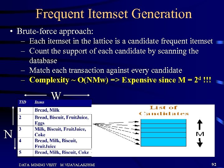Frequent Itemset Generation • Brute-force approach: – Each itemset in the lattice is a candidate frequent itemset – Count the support of each candidate by scanning the database – Match each transaction against every candidate – Complexity ~ O(NMw) => Expensive since M = 2 d !!! W N DATA MINING VESIT M. VIJAYALAKSHMI 92

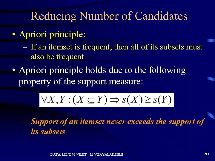Reducing Number of Candidates • Apriori principle: – If an itemset is frequent, then all of its subsets must also be frequent • Apriori principle holds due to the following property of the support measure: – Support of an itemset never exceeds the support of its subsets DATA MINING VESIT M. VIJAYALAKSHMI 93

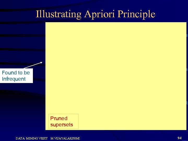Illustrating Apriori Principle Found to be Infrequent Pruned supersets DATA MINING VESIT M. VIJAYALAKSHMI 94

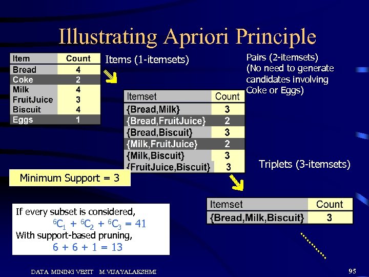Illustrating Apriori Principle Items (1 -itemsets) Pairs (2 -itemsets) (No need to generate candidates involving Coke or Eggs) Triplets (3 -itemsets) Minimum Support = 3 If every subset is considered, 6 C 1 + 6 C 2 + 6 C 3 = 41 With support-based pruning, 6 + 1 = 13 DATA MINING VESIT M. VIJAYALAKSHMI 95

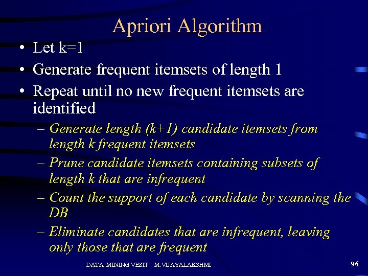Apriori Algorithm • Let k=1 • Generate frequent itemsets of length 1 • Repeat until no new frequent itemsets are identified – Generate length (k+1) candidate itemsets from length k frequent itemsets – Prune candidate itemsets containing subsets of length k that are infrequent – Count the support of each candidate by scanning the DB – Eliminate candidates that are infrequent, leaving only those that are frequent DATA MINING VESIT M. VIJAYALAKSHMI 96

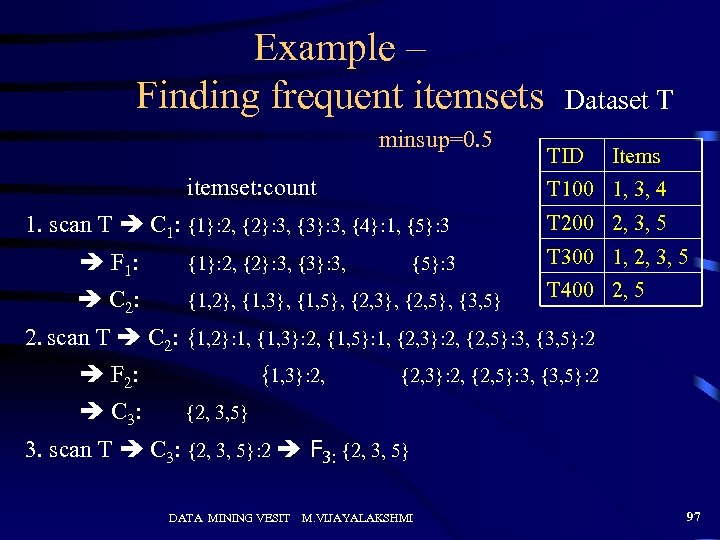Example – Finding frequent itemsets minsup=0. 5 itemset: count Dataset T TID Items T 100 1, 3, 4 1. scan T C 1: {1}: 2, {2}: 3, {3}: 3, {4}: 1, {5}: 3 F 1: {1}: 2, {2}: 3, {3}: 3, C 2: {1, 2}, {1, 3}, {1, 5}, {2, 3}, {2, 5}, {3, 5} {5}: 3 T 200 2, 3, 5 T 300 1, 2, 3, 5 T 400 2, 5 2. scan T C 2: {1, 2}: 1, {1, 3}: 2, {1, 5}: 1, {2, 3}: 2, {2, 5}: 3, {3, 5}: 2 F 2: C 3: {1, 3}: 2, {2, 3}: 2, {2, 5}: 3, {3, 5}: 2 {2, 3, 5} 3. scan T C 3: {2, 3, 5}: 2 F 3: {2, 3, 5} DATA MINING VESIT M. VIJAYALAKSHMI 97

Apriori Adv/Disadv • Advantages: – Uses large itemset property. – Easily parallelized – Easy to implement. • Disadvantages: – Assumes transaction database is memory resident. – Requires up to m database scans. DATA MINING VESIT M. VIJAYALAKSHMI 98

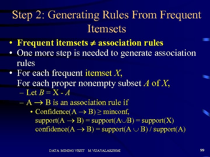Step 2: Generating Rules From Frequent Itemsets • Frequent itemsets association rules • One more step is needed to generate association rules • For each frequent itemset X, For each proper nonempty subset A of X, – Let B = X - A – A B is an association rule if • Confidence(A B) ≥ minconf, support(A B) = support(A B) = support(X) confidence(A B) = support(A B) / support(A) DATA MINING VESIT M. VIJAYALAKSHMI 99

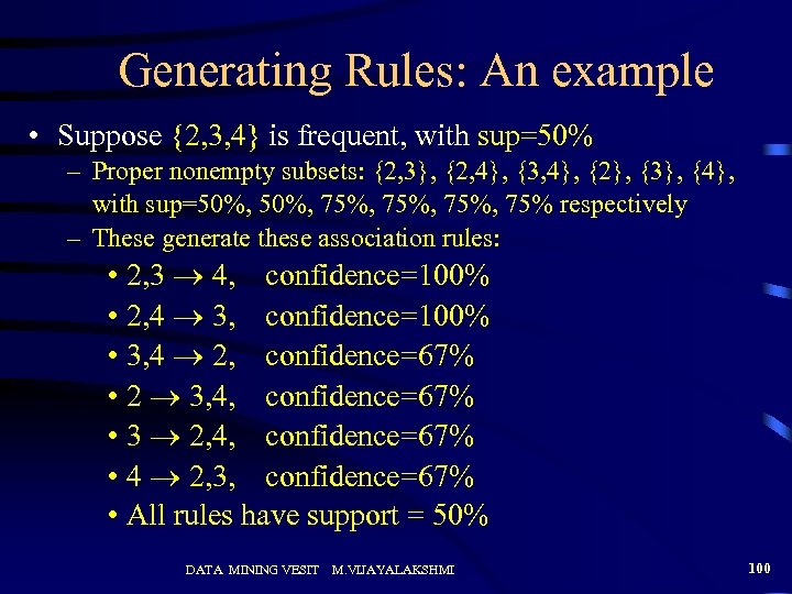Generating Rules: An example • Suppose {2, 3, 4} is frequent, with sup=50% – Proper nonempty subsets: {2, 3}, {2, 4}, {3, 4}, {2}, {3}, {4}, with sup=50%, 75%, 75% respectively – These generate these association rules: • 2, 3 4, confidence=100% • 2, 4 3, confidence=100% • 3, 4 2, confidence=67% • 2 3, 4, confidence=67% • 3 2, 4, confidence=67% • 4 2, 3, confidence=67% • All rules have support = 50% DATA MINING VESIT M. VIJAYALAKSHMI 100

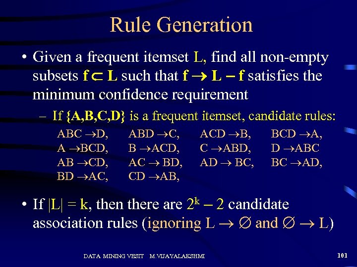Rule Generation • Given a frequent itemset L, find all non-empty subsets f L such that f L – f satisfies the minimum confidence requirement – If {A, B, C, D} is a frequent itemset, candidate rules: ABC D, A BCD, AB CD, BD AC, ABD C, B ACD, AC BD, CD AB, ACD B, C ABD, AD BC, BCD A, D ABC BC AD, • If |L| = k, then there are 2 k – 2 candidate association rules (ignoring L and L) DATA MINING VESIT M. VIJAYALAKSHMI 101

Generating Rules • To recap, in order to obtain A B, we need to have support(A B) and support(A) • All the required information for confidence computation has already been recorded in itemset generation. No need to see the data T any more. • This step is not as time-consuming as frequent itemsets generation. DATA MINING VESIT M. VIJAYALAKSHMI 102

Rule Generation • How to efficiently generate rules from frequent itemsets? – In general, confidence does not have an antimonotone property c(ABC D) can be larger or smaller than c(AB D) – But confidence of rules generated from the same itemset has an anti-monotone property – e. g. , L = {A, B, C, D}: c(ABC D) c(AB CD) c(A BCD) DATA MINING VESIT M. VIJAYALAKSHMI 103

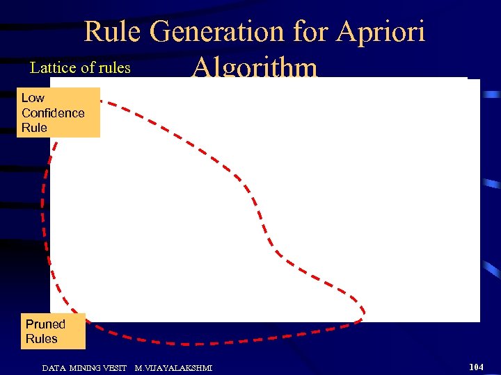Rule Generation for Apriori Lattice of rules Algorithm Low Confidence Rule Pruned Rules DATA MINING VESIT M. VIJAYALAKSHMI 104

Rule Generation for Apriori Algorithm • Candidate rule is generated by merging two rules that share the same prefix in the rule consequent • Join (CD=>AB, BD=>AC) would produce the candidate rule D => ABC • Prune rule D=>ABC if its subset AD=>BC does not have high confidence DATA MINING VESIT M. VIJAYALAKSHMI 105

APriori - Performance Bottlenecks • The core of the Apriori algorithm: – Use frequent (k – 1)-itemsets to generate candidate frequent k -itemsets – Use database scan and pattern matching to collect counts for the candidate itemsets • Bottleneck of Apriori: candidate generation – Huge candidate sets: • 104 frequent 1 -itemset will generate 107 candidate 2 itemsets • To discover a frequent pattern of size 100, e. g. , {a 1, a 2, …, a 100}, one needs to generate 2100 1030 candidates. – Multiple scans of database: • Needs (n +1 ) scans, n is the length of the longest pattern DATA MINING VESIT M. VIJAYALAKSHMI 106

Mining Frequent Patterns Without Candidate Generation • Compress a large database into a compact, Frequent. Pattern tree (FP-tree) structure – highly condensed, but complete for frequent pattern mining – avoid costly database scans • Develop an efficient, FP-tree-based frequent pattern mining method – A divide-and-conquer methodology: decompose mining tasks into smaller ones – Avoid candidate generation: sub-database test only! DATA MINING VESIT M. VIJAYALAKSHMI 107

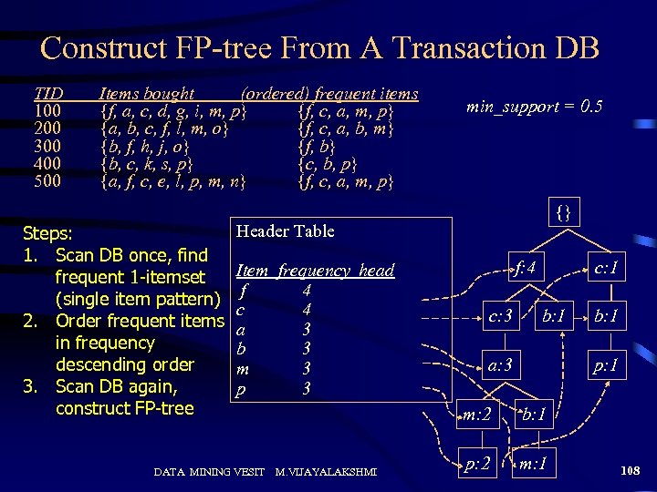Construct FP-tree From A Transaction DB TID 100 200 300 400 500 Items bought (ordered) frequent items {f, a, c, d, g, i, m, p} {f, c, a, m, p} {a, b, c, f, l, m, o} {f, c, a, b, m} {b, f, h, j, o} {f, b} {b, c, k, s, p} {c, b, p} {a, f, c, e, l, p, m, n} {f, c, a, m, p} Steps: 1. Scan DB once, find frequent 1 -itemset (single item pattern) 2. Order frequent items in frequency descending order 3. Scan DB again, construct FP-tree min_support = 0. 5 {} Header Table Item frequency head f 4 c 4 a 3 b 3 m 3 p 3 DATA MINING VESIT f: 4 c: 3 c: 1 b: 1 a: 3 p: 1 m: 2 M. VIJAYALAKSHMI b: 1 p: 2 m: 1 108

Benefits of the FP-tree Structure • Completeness: – never breaks a long pattern of any transaction – preserves complete information for frequent pattern mining • Compactness – reduce irrelevant information—infrequent items are gone – frequency descending ordering: more frequent items are more likely to be shared – never be larger than the original database (if not count nodelinks and counts) DATA MINING VESIT M. VIJAYALAKSHMI 109

Mining Frequent Patterns Using FP-tree • General idea (divide-and-conquer) – Recursively grow frequent pattern path using the FP-tree • Method – For each item, construct its conditional pattern-base, and then its conditional FP-tree – Repeat the process on each newly created conditional FPtree – Until the resulting FP-tree is empty, or it contains only one path (single path will generate all the combinations of its sub-paths, each of which is a frequent pattern) DATA MINING VESIT M. VIJAYALAKSHMI 110

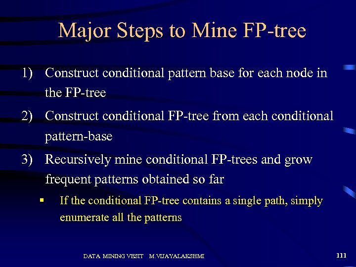Major Steps to Mine FP-tree 1) Construct conditional pattern base for each node in the FP-tree 2) Construct conditional FP-tree from each conditional pattern-base 3) Recursively mine conditional FP-trees and grow frequent patterns obtained so far § If the conditional FP-tree contains a single path, simply enumerate all the patterns DATA MINING VESIT M. VIJAYALAKSHMI 111

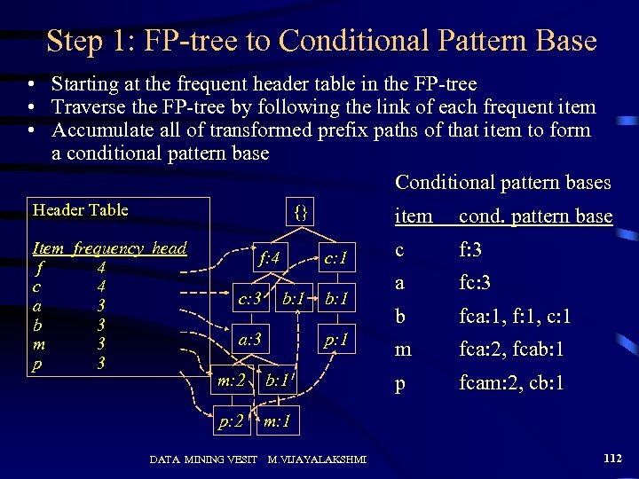Step 1: FP-tree to Conditional Pattern Base • Starting at the frequent header table in the FP-tree • Traverse the FP-tree by following the link of each frequent item • Accumulate all of transformed prefix paths of that item to form a conditional pattern base Conditional pattern bases Header Table {} Item frequency head f 4 c 4 a 3 b 3 m 3 p 3 f: 4 c: 3 item c: 1 b: 1 a: 3 b: 1 p: 1 m: 2 b: 1 p: 2 cond. pattern base c f: 3 a fc: 3 b fca: 1, f: 1, c: 1 m fca: 2, fcab: 1 p fcam: 2, cb: 1 m: 1 DATA MINING VESIT M. VIJAYALAKSHMI 112

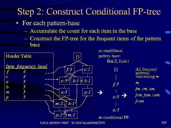Step 2: Construct Conditional FP-tree • For each pattern-base – Accumulate the count for each item in the base – Construct the FP-tree for the frequent items of the pattern base Header Table m-conditional pattern base: fca: 2, fcab: 1 {} Item frequency head f 4 c 4 a 3 b 3 m 3 p 3 f: 4 c: 3 b: 1 a: 3 m: 2 p: 2 {} c: 1 b: 1 p: 1 f: 3 c: 3 b: 1 m: 1 DATA MINING VESIT All frequent patterns concerning m m, fm, cm, am, fcm, fam, cam, fcam a: 3 m-conditional FPM. VIJAYALAKSHMI tree 113

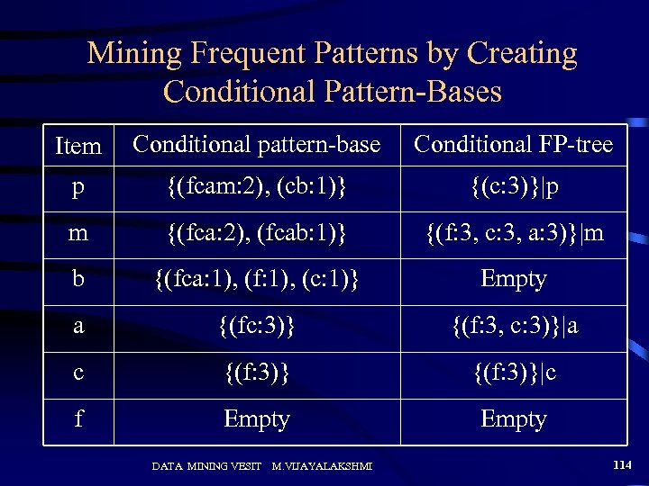Mining Frequent Patterns by Creating Conditional Pattern-Bases Item Conditional pattern-base Conditional FP-tree p {(fcam: 2), (cb: 1)} {(c: 3)}|p m {(fca: 2), (fcab: 1)} {(f: 3, c: 3, a: 3)}|m b {(fca: 1), (f: 1), (c: 1)} Empty a {(fc: 3)} {(f: 3, c: 3)}|a c {(f: 3)}|c f Empty DATA MINING VESIT M. VIJAYALAKSHMI 114

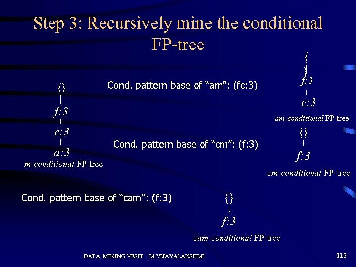Step 3: Recursively mine the conditional FP-tree { } f: 3 Cond. pattern base of “am”: (fc: 3) {} c: 3 f: 3 am-conditional FP-tree c: 3 {} Cond. pattern base of “cm”: (f: 3) a: 3 m-conditional FP-tree f: 3 cm-conditional FP-tree {} Cond. pattern base of “cam”: (f: 3) f: 3 cam-conditional FP-tree DATA MINING VESIT M. VIJAYALAKSHMI 115

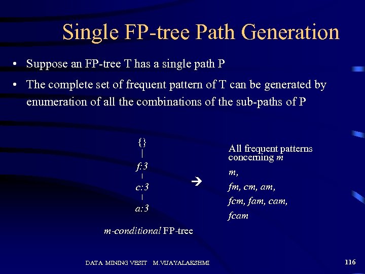Single FP-tree Path Generation • Suppose an FP-tree T has a single path P • The complete set of frequent pattern of T can be generated by enumeration of all the combinations of the sub-paths of P {} f: 3 c: 3 a: 3 All frequent patterns concerning m m, fm, cm, am, fcm, fam, cam, fcam m-conditional FP-tree DATA MINING VESIT M. VIJAYALAKSHMI 116

Why Is Frequent Pattern Growth Fast? • Performance study shows – FP-growth is an order of magnitude faster than Apriori, and is also faster than tree-projection • Reasoning – No candidate generation, no candidate test – Use compact data structure – Eliminate repeated database scan – Basic operation is counting and FP-tree building DATA MINING VESIT M. VIJAYALAKSHMI 117