4b516666fd18adb56adb63eb0c9a71f5.ppt
- Количество слайдов: 16
Outline • Model fitting in Win. BUGS • Choosing next dose • Pre-trial simulations
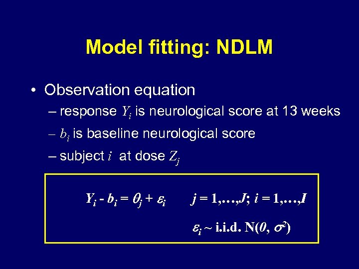
Model fitting: NDLM • Observation equation – response Yi is neurological score at 13 weeks – bi is baseline neurological score – subject i at dose Zj Yi - bi = j + i j = 1, …, J; i = 1, …, I i ~ i. i. d. N(0, 2)
![Observation equation: Win. BUGS model{ for (i in 1: I){ Y[i] ~ dnorm(mu[i], sigma Observation equation: Win. BUGS model{ for (i in 1: I){ Y[i] ~ dnorm(mu[i], sigma](https://present5.com/presentation/4b516666fd18adb56adb63eb0c9a71f5/image-3.jpg)
Observation equation: Win. BUGS model{ for (i in 1: I){ Y[i] ~ dnorm(mu[i], sigma 2 inv) mu[i] <- baseline[i] + theta[d[i]] } sampling distribution sigma 2 inv <- 1 / (sigma * sigma) sigma ~ dnorm(0, 0. 1)I(0, ) } vague, half-Normal prior on σ sampling precision θ is change from baseline specify prior
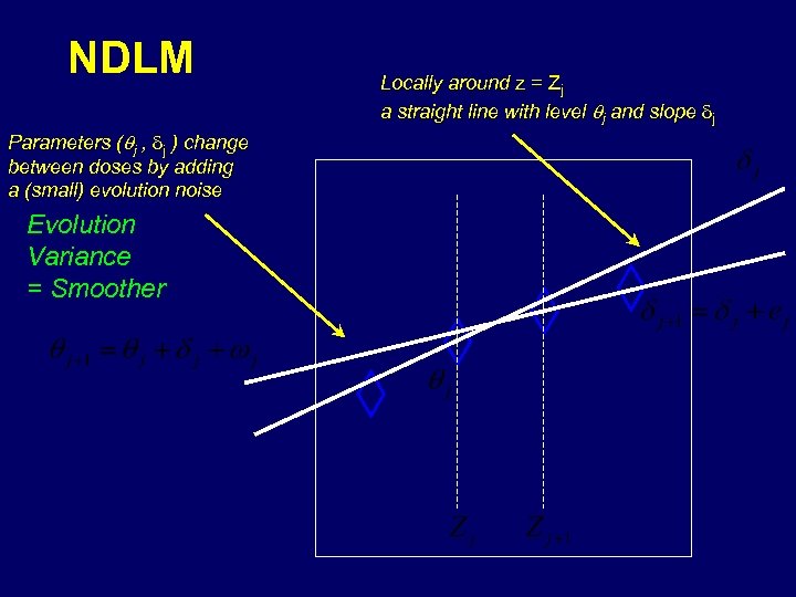
NDLM Parameters (qj , dj ) change between doses by adding a (small) evolution noise Evolution Variance = Smoother Locally around z = Zj a straight line with level qj and slope dj
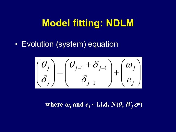
Model fitting: NDLM • Evolution (system) equation where ωj and ej ~ i. i. d. N(0, Wj 2)
![Evolution equation: Win. BUGS theta[1] ~ dnorm(mu. theta 0, prec. theta 0) delta[1] ~ Evolution equation: Win. BUGS theta[1] ~ dnorm(mu. theta 0, prec. theta 0) delta[1] ~](https://present5.com/presentation/4b516666fd18adb56adb63eb0c9a71f5/image-6.jpg)
Evolution equation: Win. BUGS theta[1] ~ dnorm(mu. theta 0, prec. theta 0) delta[1] ~ dnorm(mu. delta 0, prec. delta 0) for(j in 2: J){ theta[j] ~ dnorm(mu. theta[j], prec. theta[j]) mu. theta[j] <- theta[j-1] + delta[j-1] delta[j] ~ dnorm(delta[j-1], prec. delta[j]) random walk prec. theta[j] <- 1 / (W * sigma) prec. delta[j] <- 1 / (W * sigma) } W ~ dunif(0. 001, 1) uniform prior on W, fraction of sampling variance vague prior on placebo level and slope θ depends on previous θ and δ evolution variance of θ, δ is W * σ2
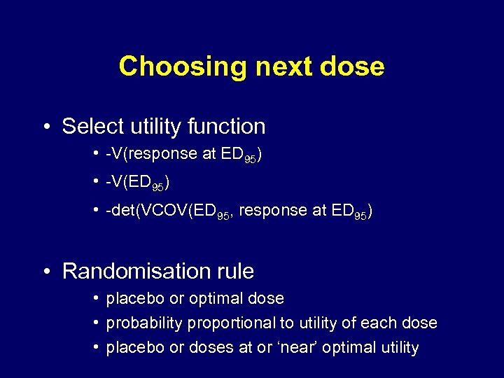
Choosing next dose • Select utility function • -V(response at ED 95) • -V(ED 95) • -det(VCOV(ED 95, response at ED 95) • Randomisation rule • placebo or optimal dose • probability proportional to utility of each dose • placebo or doses at or ‘near’ optimal utility
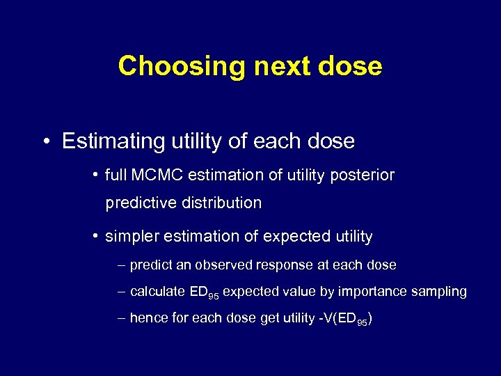
Choosing next dose • Estimating utility of each dose • full MCMC estimation of utility posterior predictive distribution • simpler estimation of expected utility – predict an observed response at each dose – calculate ED 95 expected value by importance sampling – hence for each dose get utility -V(ED 95)
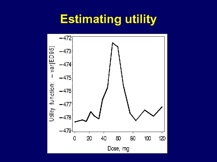
Estimating utility
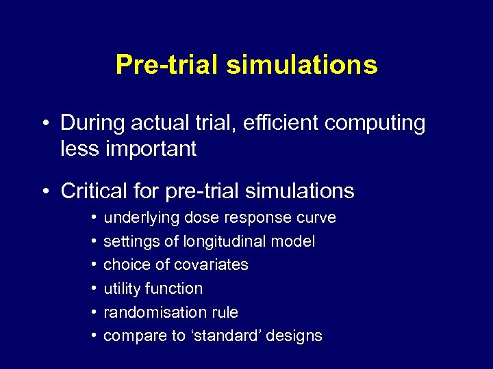
Pre-trial simulations • During actual trial, efficient computing less important • Critical for pre-trial simulations • • • underlying dose response curve settings of longitudinal model choice of covariates utility function randomisation rule compare to ‘standard’ designs
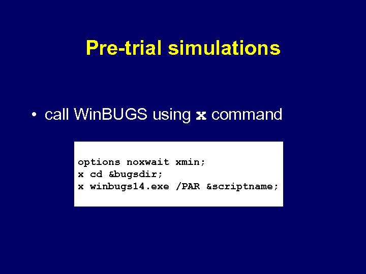
Pre-trial simulations • call Win. BUGS using x command options noxwait xmin; x cd &bugsdir; x winbugs 14. exe /PAR &scriptname;
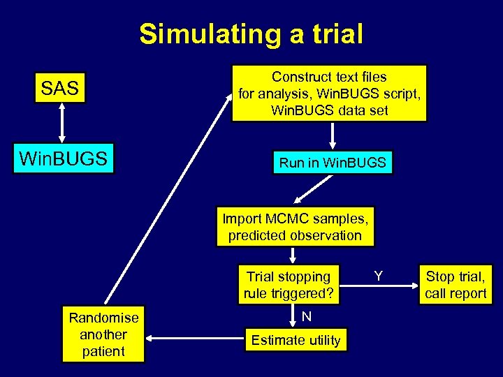
Simulating a trial SAS Construct text files for analysis, Win. BUGS script, Win. BUGS data set Win. BUGS Run in Win. BUGS Import MCMC samples, predicted observation Trial stopping rule triggered? Randomise another patient N Estimate utility Y Stop trial, call report
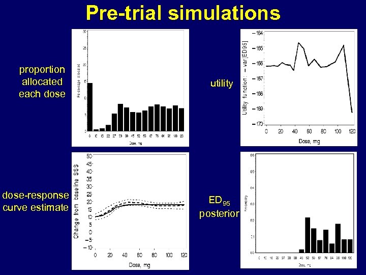
Pre-trial simulations proportion allocated each dose-response curve estimate utility ED 95 posterior
Summary • Adaptive design (NDLM) straightforward in Win. BUGS • Generic software simplifies implementation and validation • Interaction with SAS permits wide scope of pre-trial simulations • …and ease of integration with in-house reporting systems in industry

Acknowledgements • UK Medical Research Council • Pfizer Global Research & Development: Andy Grieve, Margaret Jones, Mike Smith, Mike Krams • Tessella: Tom Parke • Duke University: Peter Müller, Don Berry

4b516666fd18adb56adb63eb0c9a71f5.ppt