Orthodox Keynesianism IS-LM Model Intermediate Macroeconomics ECON-305 Spring

Orthodox Keynesianism: IS-LM Model Intermediate Macroeconomics ECON-305 Spring 2013 Professor Dalton Boise State University

Purposes 1. 2. 3. 4. Review the IS-LM Model Consider effectiveness of monetary and fiscal policy in terms of model Discuss original Phillips Curve model and importance to orthodox Keynesian analysis Summarize central propositions of orthodox Keynesianism

Recurrent Themes n Controversy over self-equilibrating properties of modern capitalist economies n Role and efficacy of activist government monetary and fiscal policy

Distinguishing Beliefs 1. Economy is inherently unstable n Subject to erratic shocks originating in business confidence 2. Economy is weakly selfequilibrating n Forces that return economy to full employment are slow and unrobust

Distinguishing Beliefs 3. Aggregate Demand determines aggregate output and employment n government can intervene to assure sufficient AD 4. Fiscal policy preferable to monetary policy n More predictable, direct and faster

Development of IS-LM J. R. Hicks, “Mr. Keynes and the Classics: A Suggested Interpretation, ” Econometrica (April, 1937) n F. Modigliani, “Liquidity Preference and the Theory of Interest and Money, ” Econometrica (January, 1944) n Popularized by A. Hansen and P. Samuelson n

IS-LM Model n IS curve represents equilibrium in the goods market n n name derives from Investment = Saving equilibrium condition LM curve represents equilibrium in the money market n name derives from Liquidity preference (Md) = Money Supply equilibrium condition

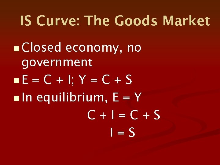IS Curve: The Goods Market n Closed economy, no government n E = C + I; Y = C + S n In equilibrium, E = Y C+I=C+S I=S

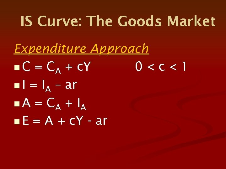IS Curve: The Goods Market Expenditure Approach n C = CA + c. Y 0

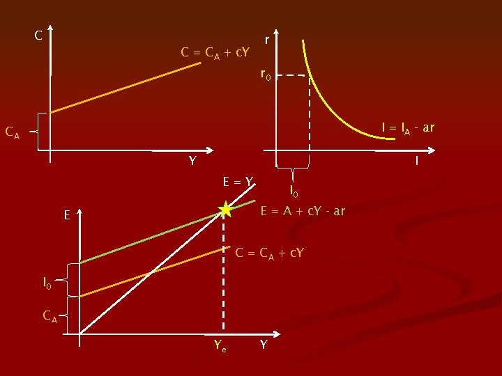C C = CA + c. Y r r 0 I = IA - ar CA Y I E=Y I 0 E = A + c. Y - ar E C = CA + c. Y I 0 CA Ye Y

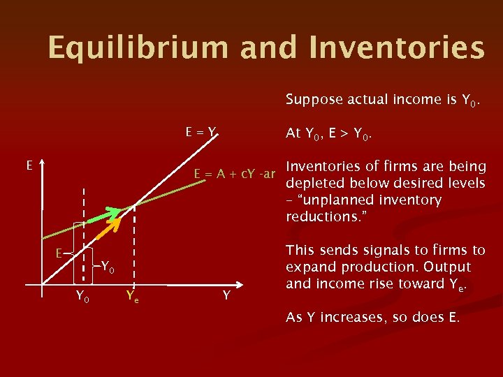Equilibrium and Inventories Suppose actual income is Y 0. E=Y E At Y 0, E > Y 0. E = A + c. Y -ar E Y 0 Ye Y Inventories of firms are being depleted below desired levels – “unplanned inventory reductions. ” This sends signals to firms to expand production. Output and income rise toward Ye. As Y increases, so does E.

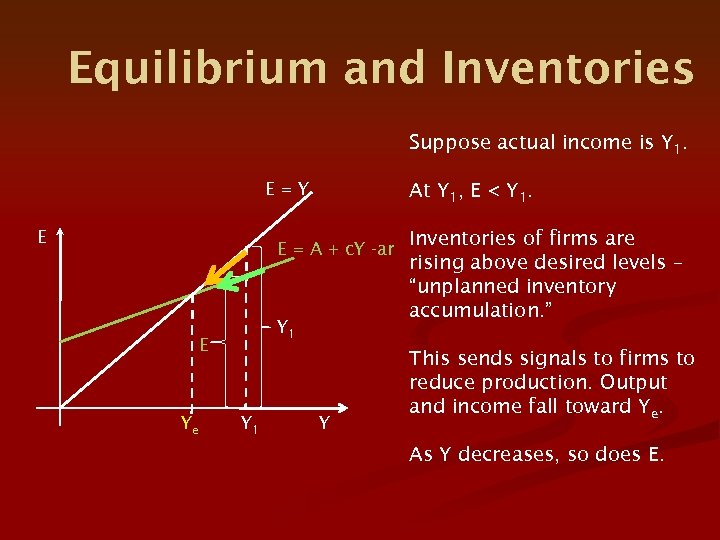Equilibrium and Inventories Suppose actual income is Y 1. E=Y E At Y 1, E < Y 1. E = A + c. Y -ar Y 1 E Ye Y 1 Y Inventories of firms are rising above desired levels – “unplanned inventory accumulation. ” This sends signals to firms to reduce production. Output and income fall toward Ye. As Y decreases, so does E.

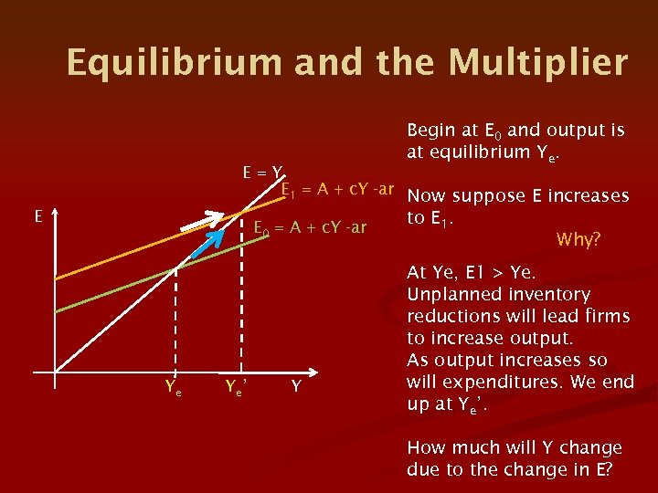Equilibrium and the Multiplier Begin at E 0 and output is at equilibrium Ye. E=Y E 1 = A + c. Y -ar Now suppose E increases E E 0 = A + c. Y -ar Ye Ye ’ Y to E 1. Why? At Ye, E 1 > Ye. Unplanned inventory reductions will lead firms to increase output. As output increases so will expenditures. We end up at Ye’. How much will Y change due to the change in E?

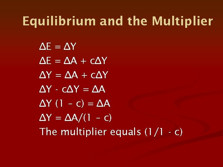Equilibrium and the Multiplier ∆E = ∆Y ∆E = ∆A + c∆Y ∆Y - c∆Y = ∆A ∆Y (1 – c) = ∆A ∆Y = ∆A/(1 – c) The multiplier equals (1/1 - c)

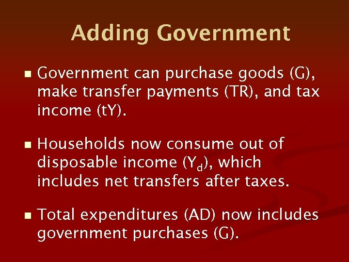Adding Government n Government can purchase goods (G), make transfer payments (TR), and tax income (t. Y). n Households now consume out of disposable income (Yd), which includes net transfers after taxes. n Total expenditures (AD) now includes government purchases (G).

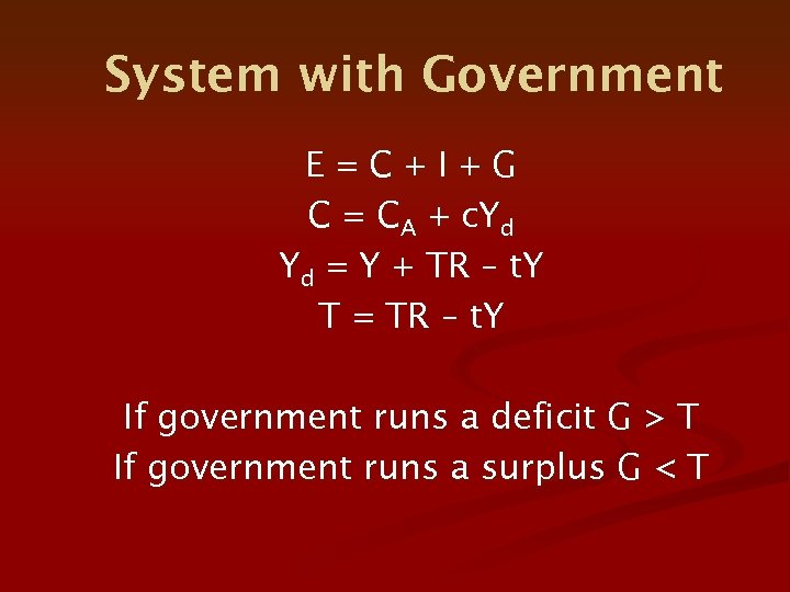System with Government E=C+I+G C = CA + c. Yd Yd = Y + TR – t. Y T = TR – t. Y If government runs a deficit G > T If government runs a surplus G < T

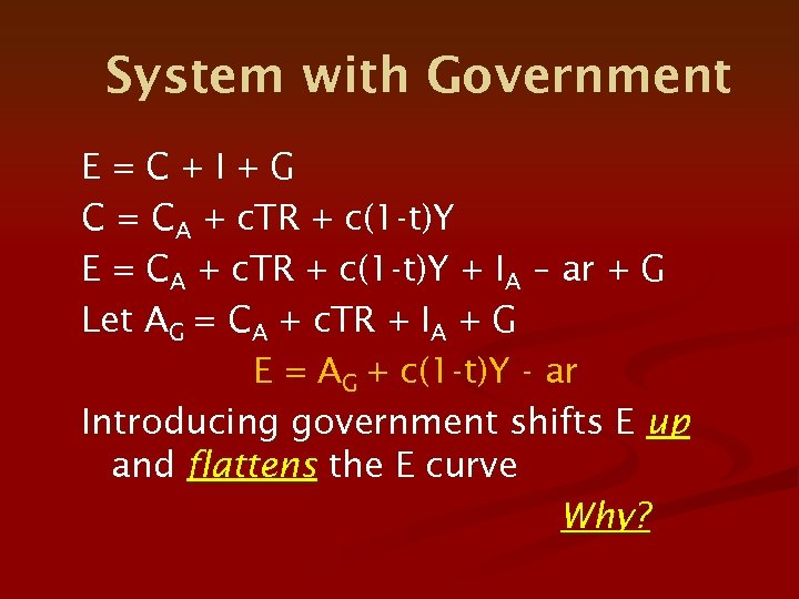System with Government E=C+I+G C = CA + c. TR + c(1 -t)Y E = CA + c. TR + c(1 -t)Y + IA – ar + G Let AG = CA + c. TR + IA + G E = AG + c(1 -t)Y - ar Introducing government shifts E up and flattens the E curve Why?

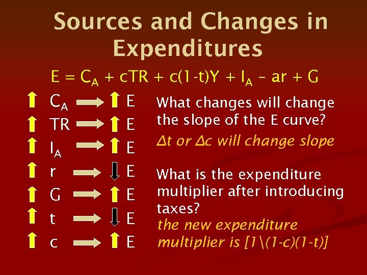Sources and Changes in Expenditures E = CA + c. TR + c(1 -t)Y + IA – ar + G CA E What changes will change TR E the slope of the E curve? ∆t or ∆c will change slope IA E r E What is the expenditure G E multiplier after introducing taxes? t E the new expenditure c E multiplier is [1(1 -c)(1 -t)]

Deriving the IS Curve

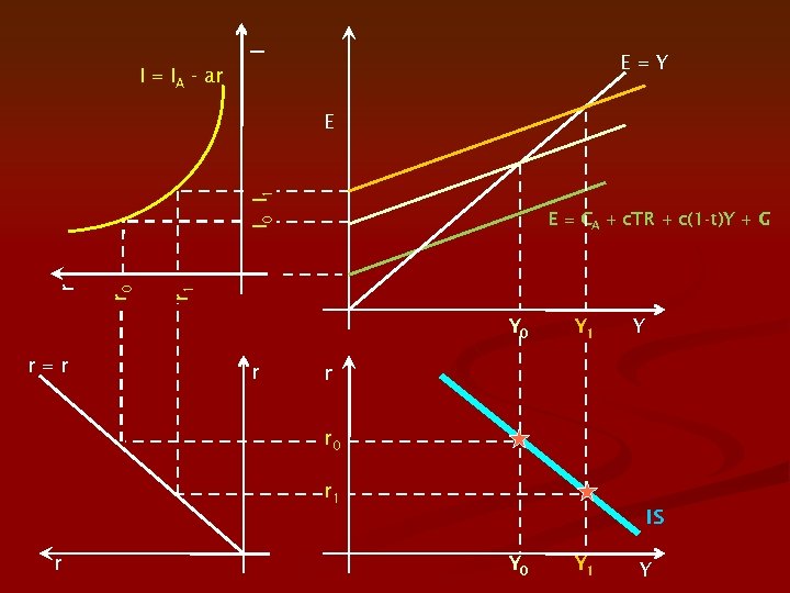I E=Y I = IA - ar E = CA + c. TR + c(1 -t)Y + G r 1 r 0 r I 0 I 1 E Y 0 r=r r Y 1 Y r r 0 r 1 IS r Y 0 Y 1 Y

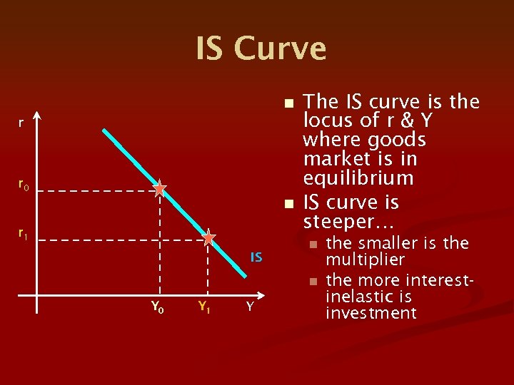IS Curve n r r 0 n r 1 IS The IS curve is the locus of r & Y where goods market is in equilibrium IS curve is steeper… n n Y 0 Y 1 Y the smaller is the multiplier the more interestinelastic is investment

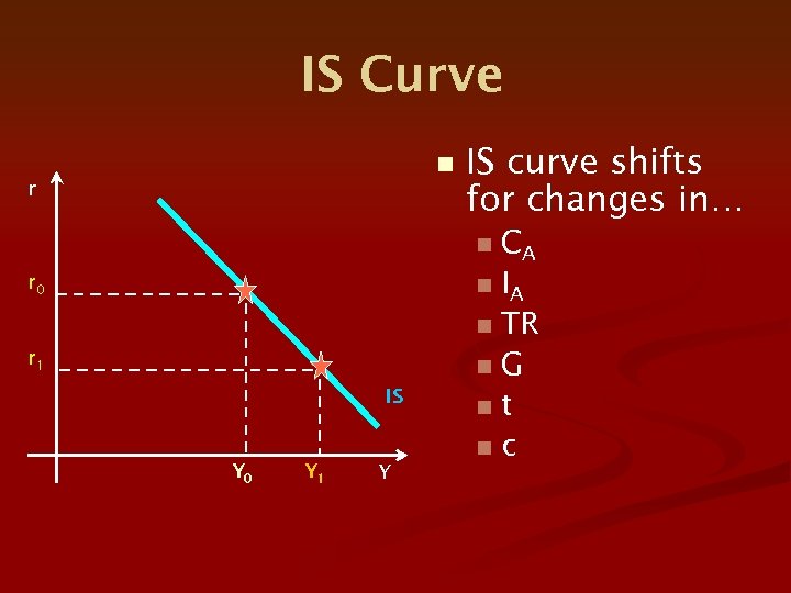IS Curve n r IS curve shifts for changes in… CA n IA n TR n. G nt nc n r 0 r 1 IS Y 0 Y 1 Y

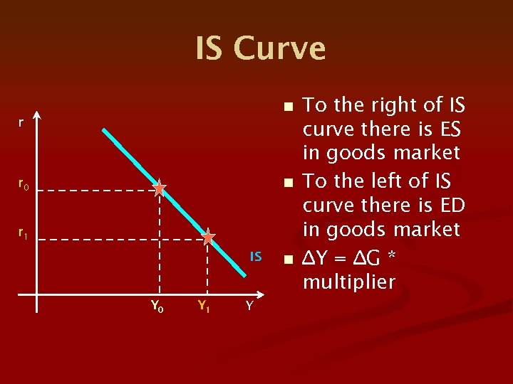IS Curve n r 0 r 1 IS Y 0 Y 1 Y n To the right of IS curve there is ES in goods market To the left of IS curve there is ED in goods market ∆Y = ∆G * multiplier

LM Curve: The Money Market n Money demand n Transactions demand. . . f(Y) n Precautionary demand … g(Y) n Speculative demand … (r v. re) n The alternative to holding money is holding securities (bonds)

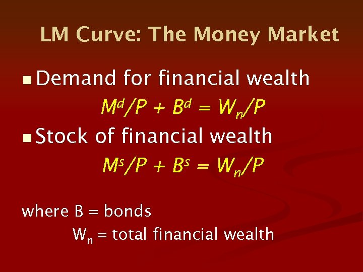LM Curve: The Money Market n Demand for financial wealth Md/P + Bd = Wn/P n Stock of financial wealth Ms/P + Bs = Wn/P where B = bonds Wn = total financial wealth

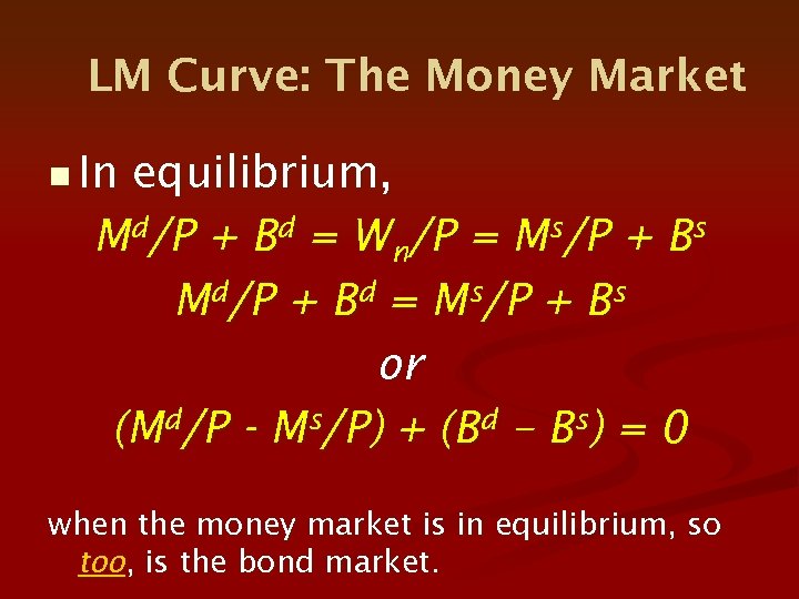LM Curve: The Money Market n In equilibrium, Md/P + Bd = Wn/P = Ms/P + Bs Md/P + Bd = Ms/P + Bs or (Md/P - Ms/P) + (Bd – Bs) = 0 when the money market is in equilibrium, so too, is the bond market.

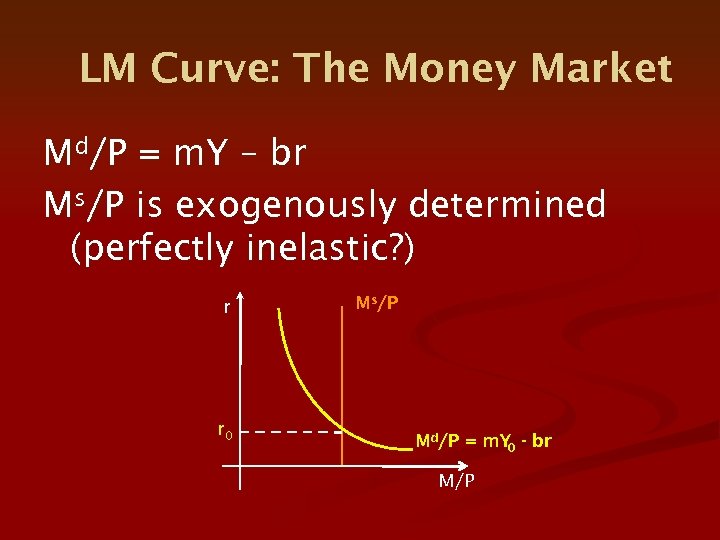LM Curve: The Money Market Md/P = m. Y – br Ms/P is exogenously determined (perfectly inelastic? ) r r 0 Ms/P Md/P = m. Y - br 0 M/P

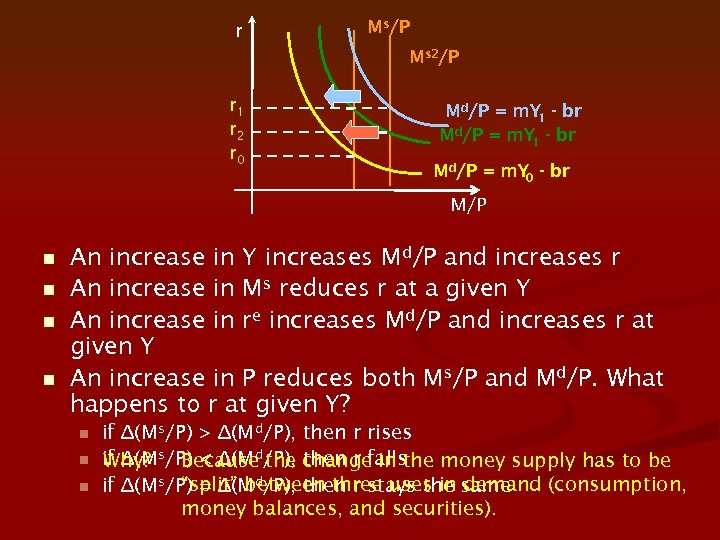r Ms/P Ms 2/P r 1 r 2 r 0 Md/P = m. Y - br 1 d/P = m. Y - br M 1 Md/P = m. Y - br 0 M/P n n An increase in Y increases Md/P and increases r An increase in Ms reduces r at a given Y An increase in re increases Md/P and increases r at given Y An increase in P reduces both Ms/P and Md/P. What happens to r at given Y? n n n if ∆(Ms/P) > ∆(Md/P), then r rises if ∆(Ms/P) < ∆(Md/P), change in the money supply has to be Why? Because then r falls “split” between three uses in demand (consumption, if ∆(Ms/P) = ∆(Md/P), then r stays the same money balances, and securities).

Deriving the LM Curve

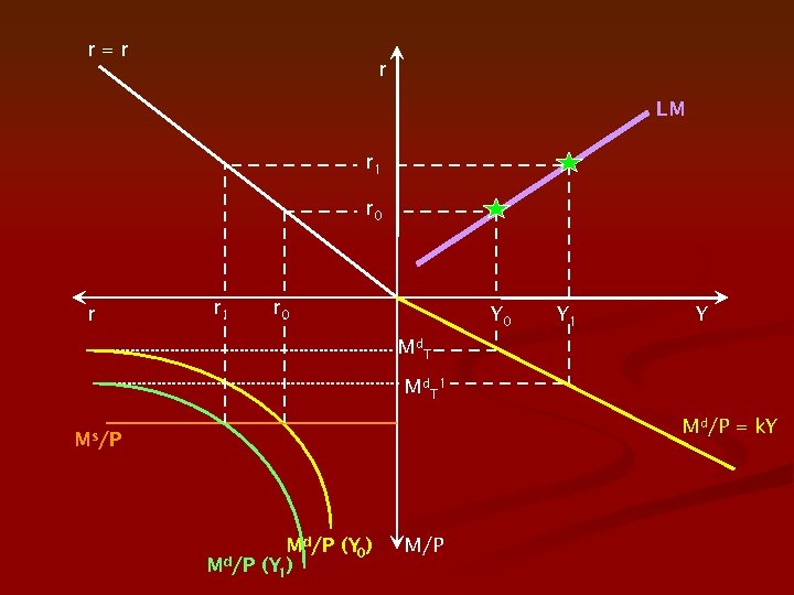r=r r LM r 1 r 0 r r 1 r 0 Y 1 Y Md T Md. T 1 Md/P = k. Y Ms/P Md/P (Y ) 0 Md/P (Y ) 1 M/P

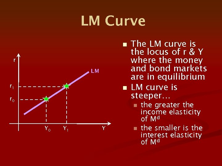LM Curve n r LM r 1 n r 0 The LM curve is the locus of r & Y where the money and bond markets are in equilibrium LM curve is steeper… n Y 0 Y 1 Y n the greater the income elasticity of Md the smaller is the interest elasticity of Md

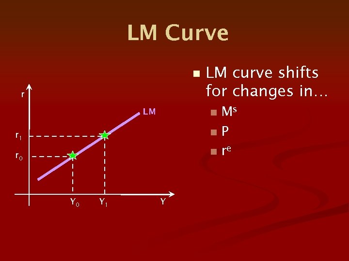LM Curve n r Ms n. P n re LM n r 1 r 0 Y 1 LM curve shifts for changes in… Y

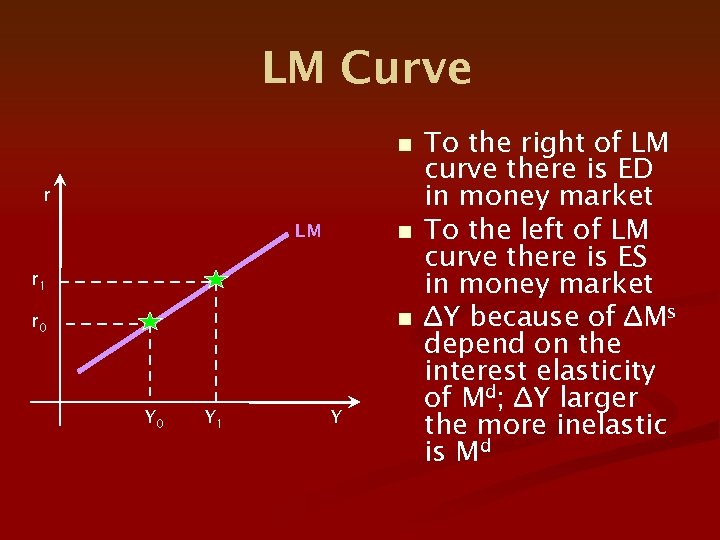LM Curve n r LM n r 1 n r 0 Y 1 Y To the right of LM curve there is ED in money market To the left of LM curve there is ES in money market ∆Y because of ∆Ms depend on the interest elasticity of Md; ∆Y larger the more inelastic is Md

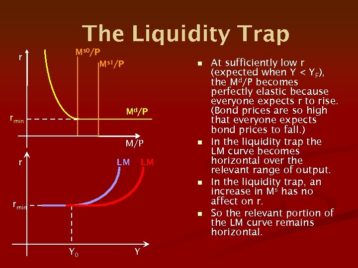The Liquidity Trap r Ms 0/P Ms 1/P n Md/P rmin M/P r LM n rmin n Y 0 Y At sufficiently low r (expected when Y < YF), the Md/P becomes perfectly elastic because everyone expects r to rise. (Bond prices are so high that everyone expects bond prices to fall. ) In the liquidity trap the LM curve becomes horizontal over the relevant range of output. In the liquidity trap, an increase in Ms has no affect on r. So the relevant portion of the LM curve remains horizontal.

What did Keynes think of his liquidity trap idea?

“There is the possibility, for the reasons discussed above, that, after the rate of interest has fallen to a certain level, liquidity-preference may become virtually absolute in the sense that almost everyone prefers cash to holding a debt which yields so low a rate of interest. In this event the monetary authority would have lost effective control over the rate of interest. But whilst this limiting case might become practically important in future, I know of no example of it hitherto. Indeed, owing to the unwillingness of most monetary authorities to deal boldly in debts of long term, there has not been much opportunity for a test. Moreover, if such a situation were to arise, it would mean that the public authority itself could borrow through the banking system on an unlimited scale at a nominal rate of interest. ” - Keynes, General Theory, p. 207

The most striking examples of a complete breakdown of stability in the rate of interest, due to the liquidity function flattening out in one direction or the other, have occurred in very abnormal circumstances. In Russia and Central Europe after the war a currency crisis or flight from the currency was experienced, when no one could be induced to retain holdings either of money or of debts on any terms whatever, and even a high and rising rate of interest was unable to keep pace with the marginal efficiency of capital (especially of stocks of liquid goods) under the influence of the expectation of an ever greater fall in the value of money; whilst in the United States at certain dates in 1932 there was a crisis of the opposite kind—a financial crisis or crisis of liquidation, when scarcely anyone could be induced to part with holdings of money on any reasonable terms. - Keynes, General Theory, p. 207

IS-LM Analytics

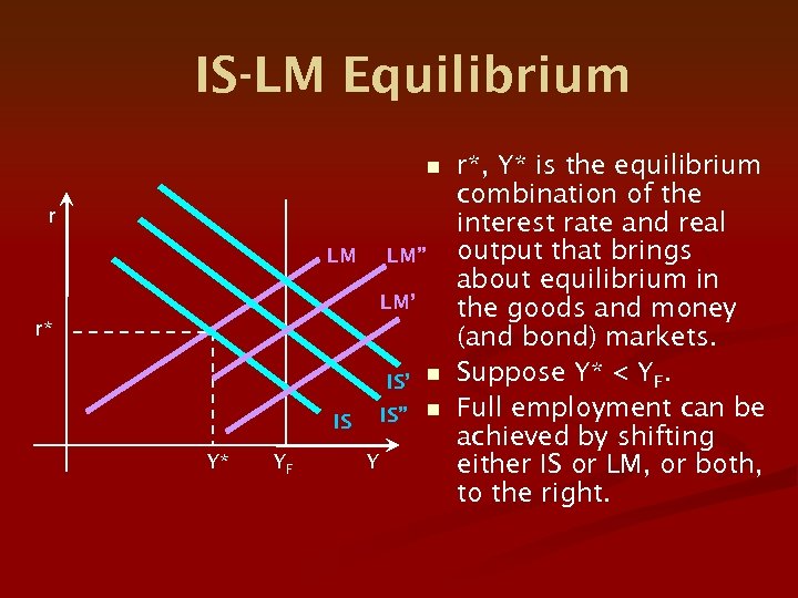IS-LM Equilibrium n r LM LM” LM’ r* IS’ n IS” n IS Y* YF Y r*, Y* is the equilibrium combination of the interest rate and real output that brings about equilibrium in the goods and money (and bond) markets. Suppose Y* < YF. Full employment can be achieved by shifting either IS or LM, or both, to the right.

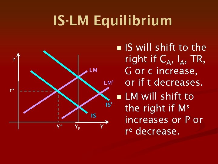IS-LM Equilibrium n r LM LM’ r* n IS’ IS Y* YF Y IS will shift to the right if CA, IA, TR, G or c increase, or if t decreases. LM will shift to the right if Ms increases or P or re decrease.

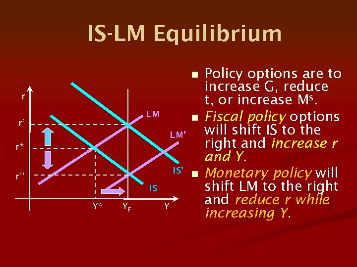IS-LM Equilibrium n r LM r’ n LM’ r* IS’ n r’’ IS Y* YF Y Policy options are to increase G, reduce t, or increase Ms. Fiscal policy options will shift IS to the right and increase r and Y. Monetary policy will shift LM to the right and reduce r while increasing Y.

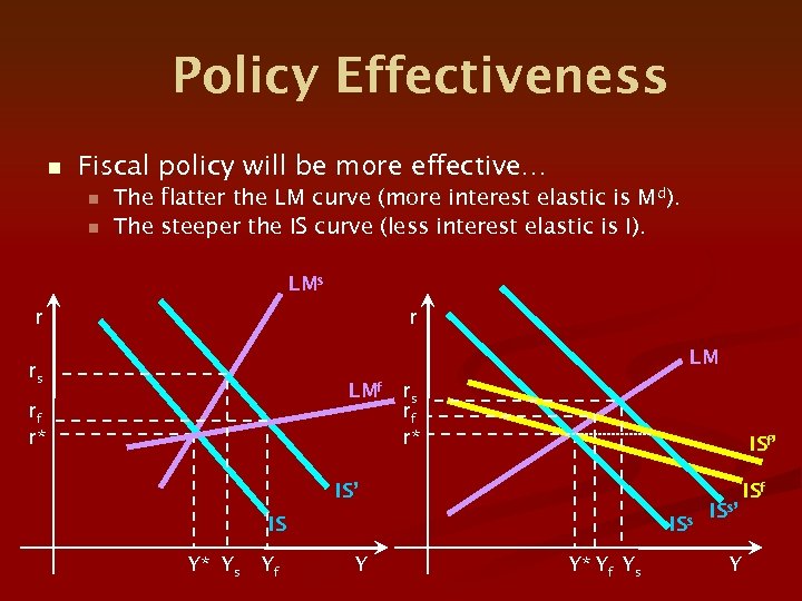Policy Effectiveness n Fiscal policy will be more effective… n n The flatter the LM curve (more interest elastic is Md). The steeper the IS curve (less interest elastic is I). LMs r r LM rs LMf rs rf r* ISf’ IS Y* Ys Yf ISs Y Y* Yf Ys ISs’ Y ISf

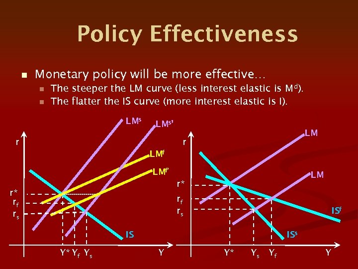Policy Effectiveness n Monetary policy will be more effective… n n The steeper the LM curve (less interest elastic is Md). The flatter the IS curve (more interest elastic is I). LMs’ r LMf LMf’ LM r* r* rf rs ISf IS Y* Yf Ys ISs Y Y* Ys Yf Y

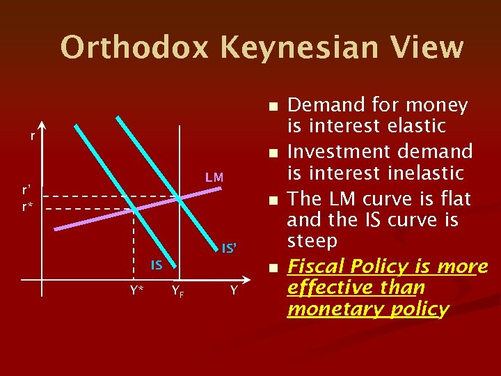Orthodox Keynesian View n r n LM r’ r* n IS’ IS Y* n YF Y Demand for money is interest elastic Investment demand is interest inelastic The LM curve is flat and the IS curve is steep Fiscal Policy is more effective than monetary policy

Policy Effectiveness n n During the 1950 s several studies sought to determine the interest elasticity of investment demand the interest elasticity of money demand. The early studies supported the Orthodox Keynesian view that investment demand was inelastic and monetary demand was elastic. The empirics supported the notion that fiscal policy was more effective than monetary policy. This empirical support, however, became increasingly questionable by the early 1960 s.

The Crowding Out Argument n n On theoretical grounds, the early 1960 s saw a questioning of the effectiveness of “pure” fiscal policy (fiscal policy unaccompanied by accommodating changes in the money supply). The argument: “Higher interest rates from expansionary fiscal policy crowd out private spending sensitive to the interest rate, limiting the effectiveness of fiscal policy. ”

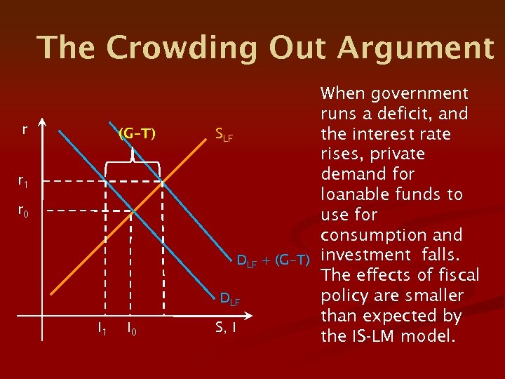The Crowding Out Argument r (G–T) r 1 r 0 I 1 I 0 When government runs a deficit, and SLF the interest rate rises, private demand for loanable funds to use for consumption and DLF + (G–T) investment falls. The effects of fiscal policy are smaller DLF than expected by S, I the IS-LM model.

The Keynesian Response n The Keynesian response to the “crowding out argument” focuses on the wealth effects of bondfinanced government expenditures n Blinder and Solow, “Does Fiscal Policy Matter? , ” Journal of Public Economics (November 1973)

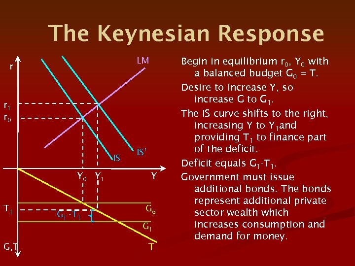The Keynesian Response LM r r 1 r 0 IS Y 0 Y 1 T 1 G 1 -T 1 IS’ Y Go G 1 G, T T Begin in equilibrium r 0, Y 0 with a balanced budget G 0 = T. Desire to increase Y, so increase G to G 1. The IS curve shifts to the right, increasing Y to Y 1 and providing T 1 to finance part of the deficit. Deficit equals G 1 -T 1. Government must issue additional bonds. The bonds represent additional private sector wealth which increases consumption and demand for money.

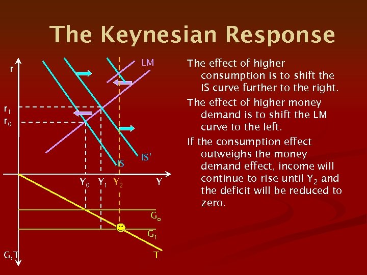The Keynesian Response LM r r 1 r 0 IS Y 0 Y 1 Y 2 IS’ Y Go G 1 G, T T The effect of higher consumption is to shift the IS curve further to the right. The effect of higher money demand is to shift the LM curve to the left. If the consumption effect outweighs the money demand effect, income will continue to rise until Y 2 and the deficit will be reduced to zero.

Debt Equivalence Theorem n n n Barro, “Are Government Bonds Net Wealth? ” Journal of Political Economy (Nov. /Dec. 1974). The burden of government spending is the same whether it is financed by an increase in taxation or by bonds. Borrowing reflects a future tax liability which if fully taken into account exactly offsets the value of the bonds in households wealth. Government Bonds are not net wealth!

Is Debt Equivalent to Taxes? n n n Are households farsighted? Do households take into account future tax liabilities that will fall on theirs? Government has privileged access to loanable funds so the interest rate at which government borrows is less than the interest rate at which future taxes are discounted. Government bonds are net wealth

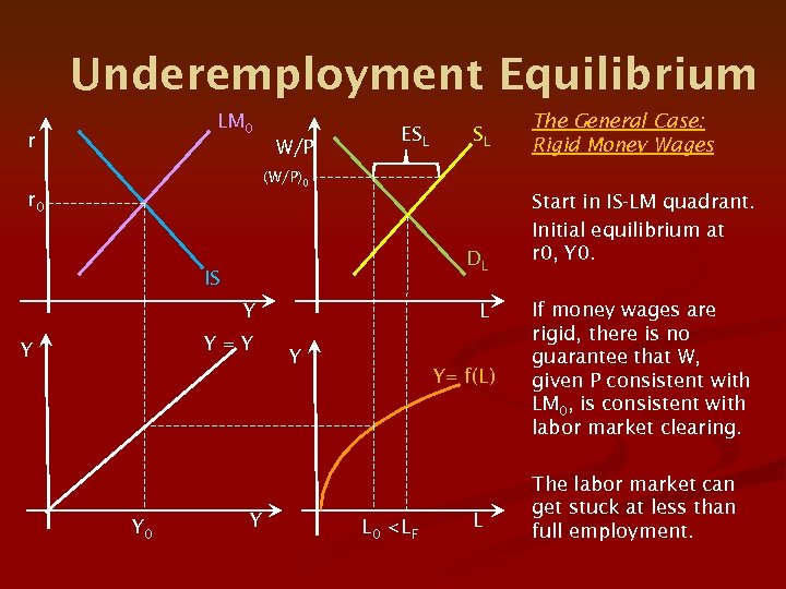Underemployment Equilibrium LM 0 r W/P ESL SL The General Case: Rigid Money Wages (W/P)0 r 0 DL IS Y Y=Y Y Y 0 Y L Y Y= f(L) L 0 < LF L Start in IS-LM quadrant. Initial equilibrium at r 0, Y 0. If money wages are rigid, there is no guarantee that W, given P consistent with LM 0, is consistent with labor market clearing. The labor market can get stuck at less than full employment.

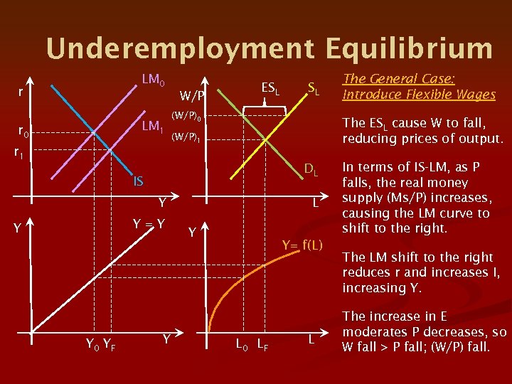Underemployment Equilibrium LM 0 r W/P LM 1 r 0 r 1 ESL (W/P)0 (W/P)1 DL Y Y=Y Y 0 YF Y The General Case: Introduce Flexible Wages The ESL cause W to fall, reducing prices of output. IS Y SL L Y Y= f(L) L 0 LF L In terms of IS-LM, as P falls, the real money supply (Ms/P) increases, causing the LM curve to shift to the right. The LM shift to the right reduces r and increases I, increasing Y. The increase in E moderates P decreases, so W fall > P fall; (W/P) fall.

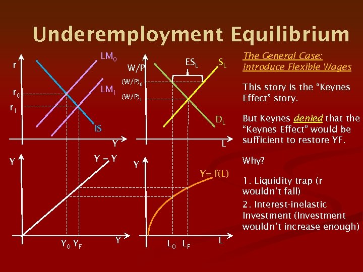Underemployment Equilibrium LM 0 r W/P LM 1 r 0 r 1 ESL (W/P)0 (W/P)1 DL Y Y=Y Y 0 YF Y The General Case: Introduce Flexible Wages This story is the “Keynes Effect” story. IS Y SL L But Keynes denied that the “Keynes Effect” would be sufficient to restore YF. Why? Y Y= f(L) L 0 LF L 1. Liquidity trap (r wouldn’t fall) 2. Interest-inelastic Investment (Investment wouldn’t increase enough)

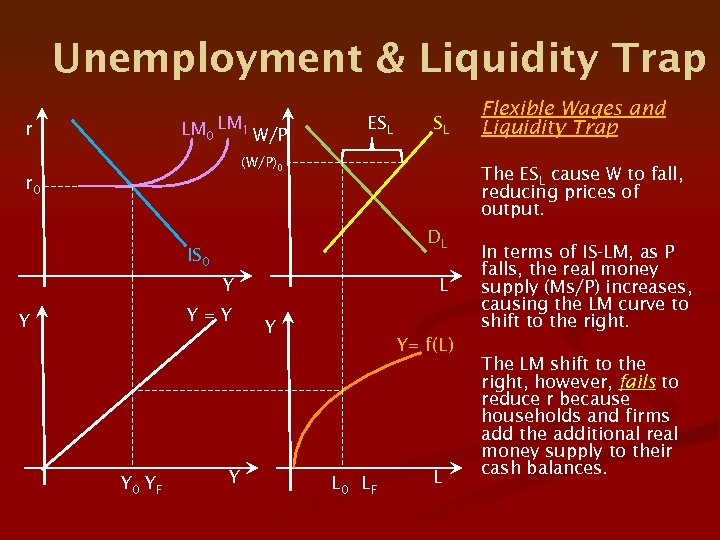Unemployment & Liquidity Trap LM 0 LM 1 W/P r ESL SL (W/P)0 r 0 The ESL cause W to fall, reducing prices of output. DL IS 0 Y Y=Y Y Y 0 YF Y Flexible Wages and Liquidity Trap L Y Y= f(L) L 0 LF L In terms of IS-LM, as P falls, the real money supply (Ms/P) increases, causing the LM curve to shift to the right. The LM shift to the right, however, fails to reduce r because households and firms add the additional real money supply to their cash balances.

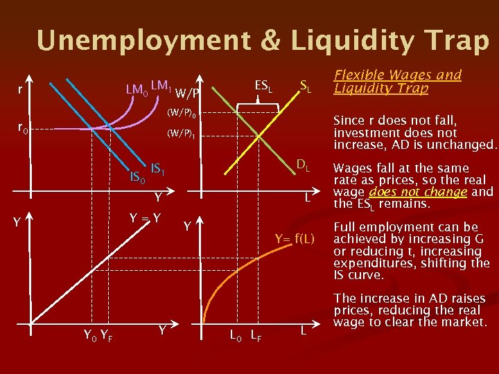Unemployment & Liquidity Trap LM 0 LM 1 W/P r ESL SL (W/P)0 r 0 Since r does not fall, investment does not increase, AD is unchanged. (W/P)1 IS 1 DL Y IS 0 L Y=Y Y Y 0 YF Y Flexible Wages and Liquidity Trap Y Y= f(L) L 0 LF L Wages fall at the same rate as prices, so the real wage does not change and the ESL remains. Full employment can be achieved by increasing G or reducing t, increasing expenditures, shifting the IS curve. The increase in AD raises prices, reducing the real wage to clear the market.

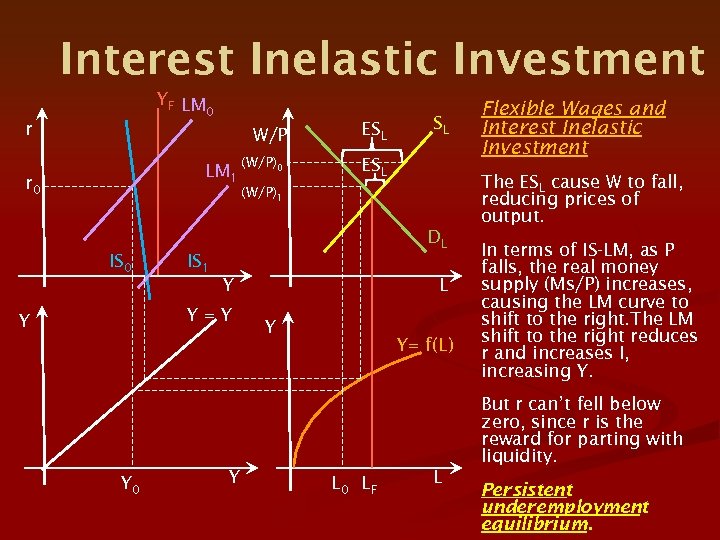Interest Inelastic Investment YF LM 0 r W/P LM 1 r 0 (W/P)0 ESL SL ESL The ESL cause W to fall, reducing prices of output. (W/P)1 DL IS 0 IS 1 Y Y=Y Y L Y Flexible Wages and Interest Inelastic Investment Y= f(L) In terms of IS-LM, as P falls, the real money supply (Ms/P) increases, causing the LM curve to shift to the right. The LM shift to the right reduces r and increases I, increasing Y. But r can’t fell below zero, since r is the reward for parting with liquidity. Y 0 Y L 0 LF L Persistent underemployment equilibrium.

Summary Orthodox Keynesian IS-LM

Orthodox Keynesian IS-LM 1. 2. 3. Rigidity of nominal wages prevent adjustment to full employment. If nominal wages are flexible, reductions in wages and prices fail to restore full employment unless the Keynes effect is operative. If liquidity trap or interest-inelastic investment exists, the Keynes Effect is short-circuited and the economy, left to itself, fails to restore full employment.

Orthodox Keynesian IS-LM Keynes failed to provide a general theory of unemployment; his argument rests on special cases (nominal wage rigidity, liquidity trap, or severe interestinelastic investment).

Wealth Effects: Real Balance and Pigou Effects

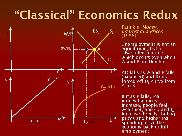“Classical” Economics Redux r ESL W/P (W/P)0 B SL A DL Y Y=Y Y Y 0 YF Y L Y Y= f(L) L 0 LF L Patinkin, Money, Interest and Prices (1956) Unemployment is not an equilibrium, but a disequilibrium one which occurs even when W and P are flexible. AD falls as W and P falls (balanced) and firms forced off DL curve from A to B. But as P falls, real money balances increase, people feel wealthier, and CA and IA increase directly. Falling prices and higher real spending move the economy back to full employment.

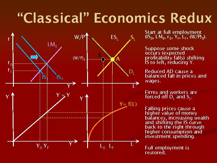“Classical” Economics Redux r W/P ESL SL LM 0 (W/P)0 r 1 IS 1 B Y Y=Y Y Y 0 YF Suppose some shock occurs (expected profitability falls) shifting IS to left, reducing Y. A DL IS 0 Y Start at full employment (IS 0, LM 0, r 0, YF, LF, (W/P)0). L Reduced AD cause a balanced fall in prices and wages. Firms and workers are forced off DL and SL. Y Y= f(L) L 0 LF L Falling prices cause a higher value of money balances, increasing wealth and shifting the IS curve back to the right through higher consumption and investment spending. Full employment is restored.

Pigou Effect n n n Patinkin’s argument concerning the “real balance effect” indirectly revives the Pigou effect argument. Pigou had argued that reduced prices increase wealth and increase AD, so that the Keynes Effect of a shifting LM curve was accompanied by a shifting IS curve to restore full employment, and that even if the Keynes Effect was inoperative, wealth effects restore equilibrium. Harry Johnson: “The Pigou effect finally disposes of the Keynesian contention that underemployment equilibrium does not depend upon the assumption of wage rigidity. It does. ”

Criticisms of Pigou Effect n n Falling prices might lead to expectations of further declines in prices, postponing consumption and delaying return to full employment. Falling prices might lead to firms delaying investment, believing recession will continue, and delay return to full employment. How does Pigou effect change wealth? Currency (outside money), Bank credit (inside money), government bonds? Empirical evidence for Pigou effect is weak.

The Neoclassical Synthesis n n n By mid-1960 s, economists widely accepted the “neoclassical synthesis. ” Keynes was wrong in terms of theory. Keynesian economics was a special case of the more general classical theory (wage rigidity). Keynes was right in terms of policy. Slow Keynes and Pigou effect adjustments mean that activist government policy is necessary.

Open Economy IS-LM

Open Economy n n Late 1950 s and early 1960 s saw increasingly liberalized (freer) trade and capital movements IS/LM extended to cover open economies n n E = Y = C + I + G + (X-Im) Exports (X) and Imports (Im) Mundell, “Capital Mobility and Stabilization Policy under Fixed and Flexible Exchange Rates, Canadian Journal of Economics and Political Science (Nov. 1963) Fleming, “Domestic Financial Policies under Fixed and under Floating Exchange Rates, ” IMF Staff Papers (Nov. 1962)

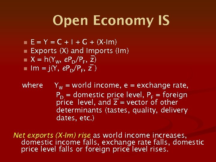Open Economy IS n n E = Y = C + I + G + (X-Im) Exports (X) and Imports (Im) X = h(YW, e. PD/PF, z) Im = j(Y, e. PD/PF, z ) where YW = world income, e = exchange rate, PD = domestic price level, PF = foreign price level, and z = vector of other determinants (tastes, quality, delivery dates, etc. ) Net exports (X-Im) rise as world income increases, domestic income falls, exchange rate falls, domestic price level falls or foreign price level rises.

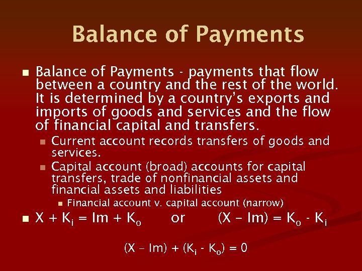Balance of Payments n Balance of Payments - payments that flow between a country and the rest of the world. It is determined by a country’s exports and imports of goods and services and the flow of financial capital and transfers. n n Current account records transfers of goods and services. Capital account (broad) accounts for capital transfers, trade of nonfinancial assets and liabilities n n Financial account v. capital account (narrow) X + Ki = Im + Ko or (X – Im) = Ko - Ki (X – Im) + (Ki - Ko) = 0

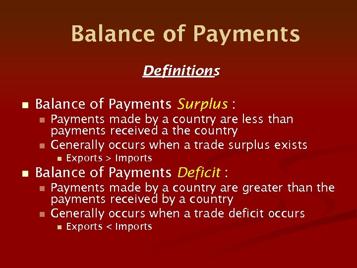Balance of Payments Definitions n Balance of Payments Surplus : n n Payments made by a country are less than payments received a the country Generally occurs when a trade surplus exists n n Exports > Imports Balance of Payments Deficit : n n Payments made by a country are greater than the payments received by a country Generally occurs when a trade deficit occurs n Exports < Imports

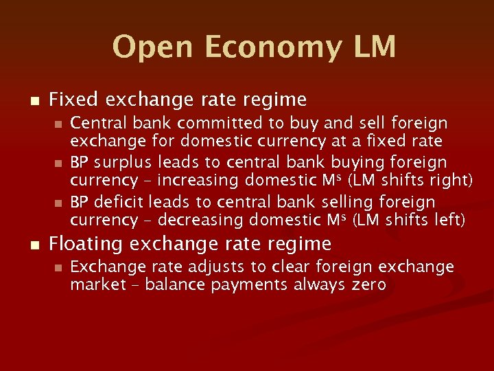Open Economy LM n Fixed exchange rate regime n n Central bank committed to buy and sell foreign exchange for domestic currency at a fixed rate BP surplus leads to central bank buying foreign currency – increasing domestic Ms (LM shifts right) BP deficit leads to central bank selling foreign currency – decreasing domestic Ms (LM shifts left) Floating exchange rate regime n Exchange rate adjusts to clear foreign exchange market – balance payments always zero

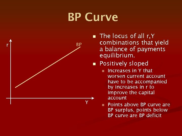BP Curve n r BP n The locus of all r, Y combinations that yield a balance of payments equilibrium. Positively sloped n Y n Increases in Y that worsen current account have to be accompanied by increases in r to improve the capital account Points above BP curve are BP surplus, points below BP curve are BP deficit

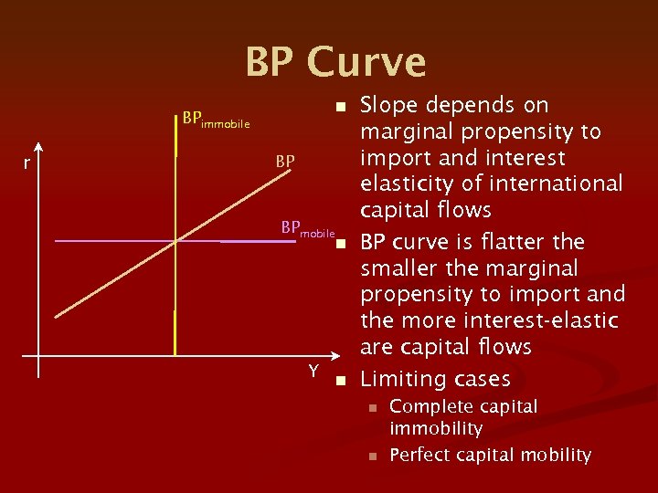BP Curve n BPimmobile r BP BPmobile n Y n Slope depends on marginal propensity to import and interest elasticity of international capital flows BP curve is flatter the smaller the marginal propensity to import and the more interest-elastic are capital flows Limiting cases n n Complete capital immobility Perfect capital mobility

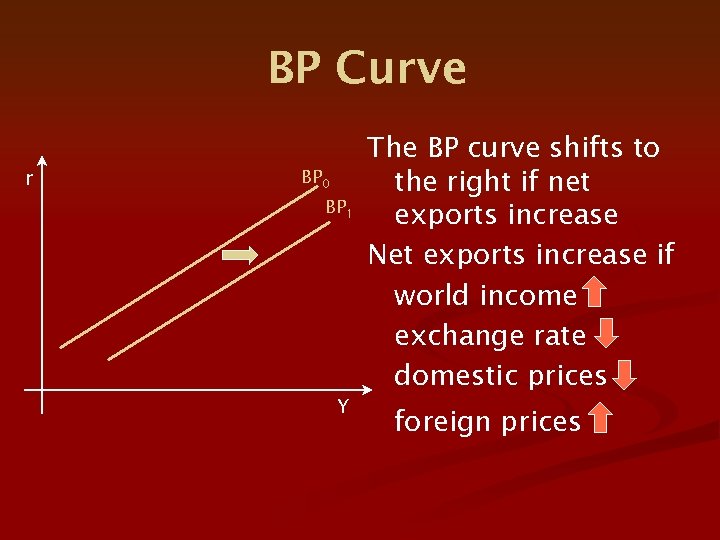BP Curve r BP 0 BP 1 Y The BP curve shifts to the right if net exports increase Net exports increase if world income exchange rate domestic prices foreign prices

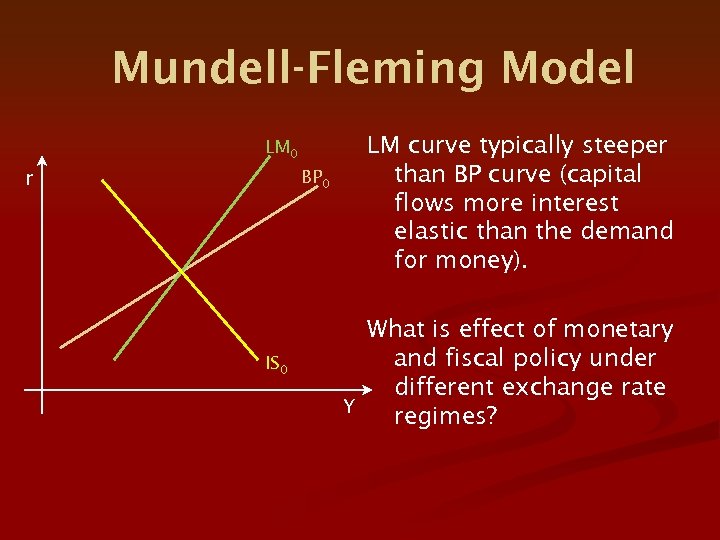Mundell-Fleming Model LM 0 BP 0 r IS 0 LM curve typically steeper than BP curve (capital flows more interest elastic than the demand for money). What is effect of monetary and fiscal policy under different exchange rate Y regimes?

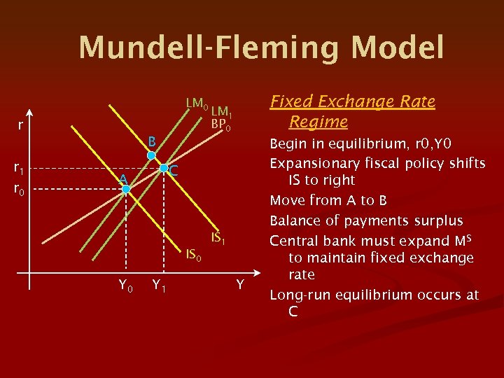Mundell-Fleming Model LM 0 r Fixed Exchange Rate Regime LM 1 BP 0 B r 1 r 0 C A IS 1 IS 0 Y 1 Y Begin in equilibrium, r 0, Y 0 Expansionary fiscal policy shifts IS to right Move from A to B Balance of payments surplus Central bank must expand MS to maintain fixed exchange rate Long-run equilibrium occurs at C

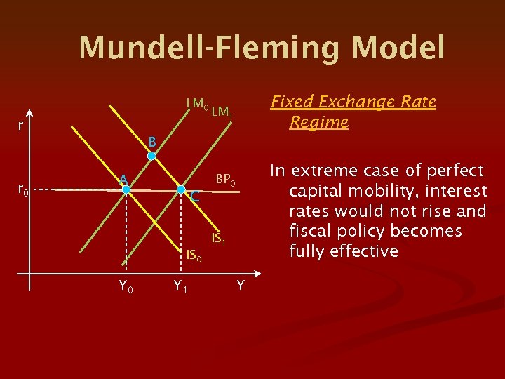Mundell-Fleming Model LM 0 r Fixed Exchange Rate Regime LM 1 B r 0 In extreme case of perfect capital mobility, interest rates would not rise and fiscal policy becomes fully effective BP 0 A C IS 1 IS 0 Y 1 Y

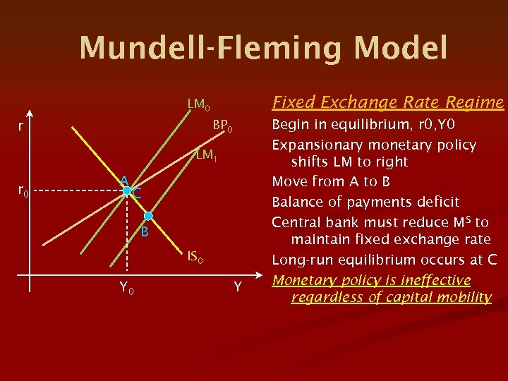Mundell-Fleming Model Fixed Exchange Rate Regime LM 0 BP 0 r LM 1 r 0 A C B IS 0 Y Begin in equilibrium, r 0, Y 0 Expansionary monetary policy shifts LM to right Move from A to B Balance of payments deficit Central bank must reduce MS to maintain fixed exchange rate Long-run equilibrium occurs at C Monetary policy is ineffective regardless of capital mobility

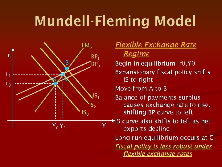Mundell-Fleming Model Flexible Exchange Rate Regime LM 0 r BP 1 BP 0 B r 1 r 0 A C IS 1 IS 2 IS 0 Y 1 Y Begin in equilibrium, r 0, Y 0 Expansionary fiscal policy shifts IS to right Move from A to B Balance of payments surplus causes exchange rate to rise, shifting BP curve to left IS curve also shifts to left as net exports decline Long-run equilibrium occurs at C Fiscal policy is less robust under flexible exchange rates

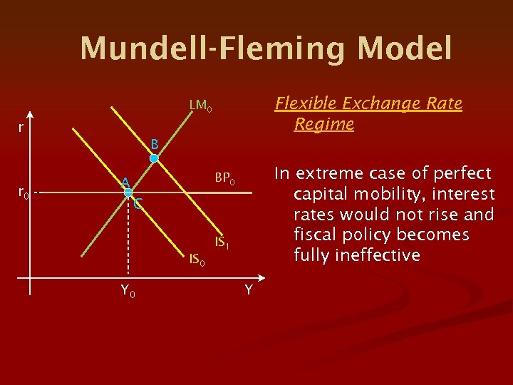Mundell-Fleming Model Flexible Exchange Rate Regime LM 0 r B r 0 In extreme case of perfect capital mobility, interest rates would not rise and fiscal policy becomes fully ineffective BP 0 A C IS 1 IS 0 Y

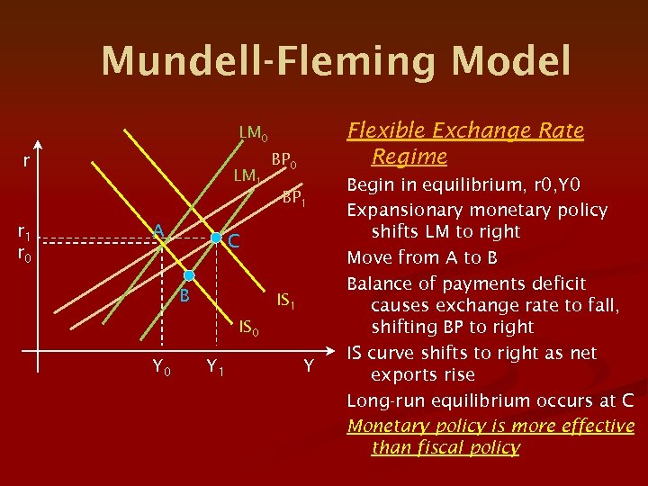Mundell-Fleming Model Flexible Exchange Rate Regime LM 0 r LM 1 BP 0 BP 1 r 0 A C B IS 1 IS 0 Y 1 Y Begin in equilibrium, r 0, Y 0 Expansionary monetary policy shifts LM to right Move from A to B Balance of payments deficit causes exchange rate to fall, shifting BP to right IS curve shifts to right as net exports rise Long-run equilibrium occurs at C Monetary policy is more effective than fiscal policy

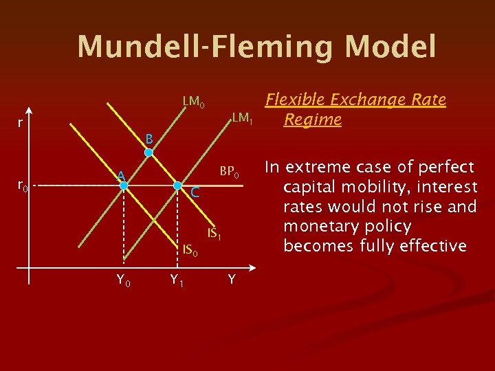Mundell-Fleming Model LM 0 LM 1 r Flexible Exchange Rate Regime B r 0 BP 0 A C IS 1 IS 0 Y 1 Y In extreme case of perfect capital mobility, interest rates would not rise and monetary policy becomes fully effective

The Phillips Curve

Original Phillips Curve n Phillips, “The Relation Between Unemployment and the Rate of Change of Money Wage Rates in the United Kingdom, 1861 -1957, ” Economica (Nov. 1958) n n Fisher, “I Discovered the Phillips Curve, ” Journal of Political Economy, (March/April 1973) [1926] Phillips found an inverse relationship between unemployment and the rate of change of money wages n Data for 1948 -1957 fit closely the earlier period 1861 -1913

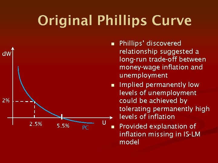Original Phillips Curve n d. W n 2% 2. 5% 5. 5% PC U n Phillips’ discovered relationship suggested a long-run trade-off between money-wage inflation and unemployment Implied permanently low levels of unemployment could be achieved by tolerating permanently high levels of inflation Provided explanation of inflation missing in IS-LM model

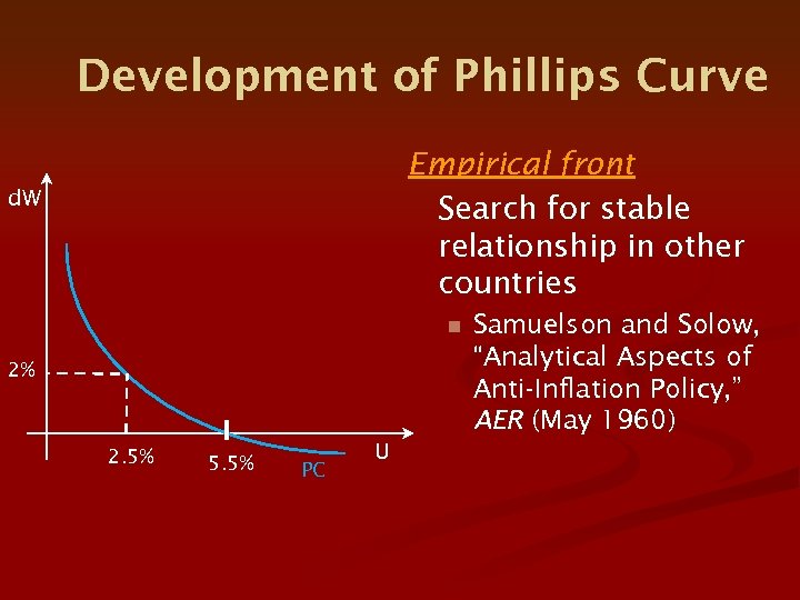Development of Phillips Curve Empirical front Search for stable relationship in other countries d. W n 2% 2. 5% 5. 5% PC U Samuelson and Solow, “Analytical Aspects of Anti-Inflation Policy, ” AER (May 1960)

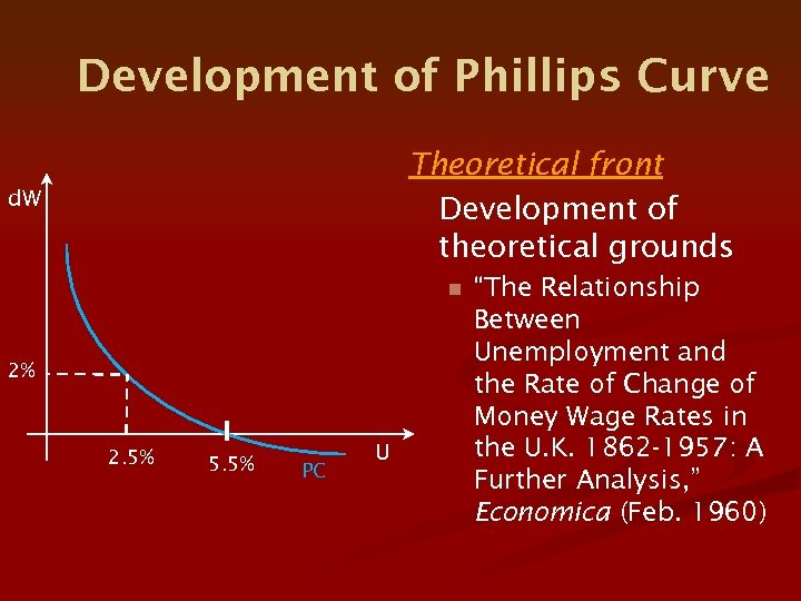Development of Phillips Curve Theoretical front Development of theoretical grounds d. W n 2% 2. 5% 5. 5% PC U “The Relationship Between Unemployment and the Rate of Change of Money Wage Rates in the U. K. 1862 -1957: A Further Analysis, ” Economica (Feb. 1960)

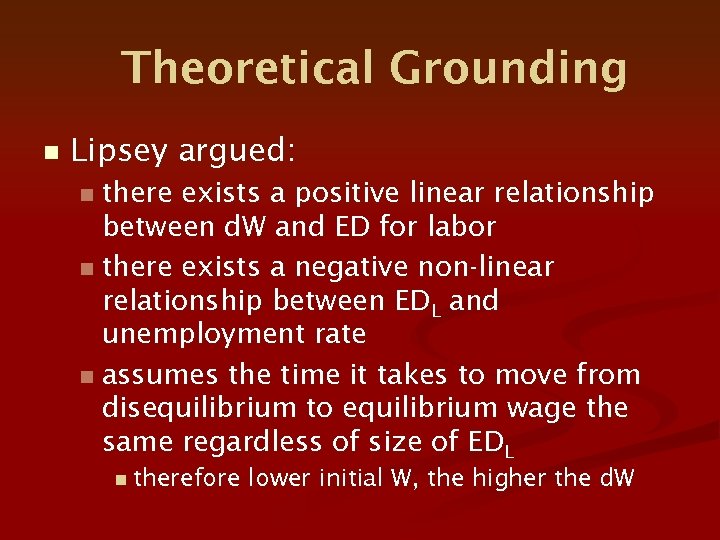Theoretical Grounding n Lipsey argued: there exists a positive linear relationship between d. W and ED for labor n there exists a negative non-linear relationship between EDL and unemployment rate n assumes the time it takes to move from disequilibrium to equilibrium wage the same regardless of size of EDL n n therefore lower initial W, the higher the d. W

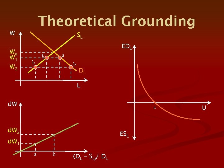Theoretical Grounding W We W 1 W 2 SL EDL a a b b DL L d. W e d. W 2 ESL d. W 1 a b (DL – SL)/ DL U

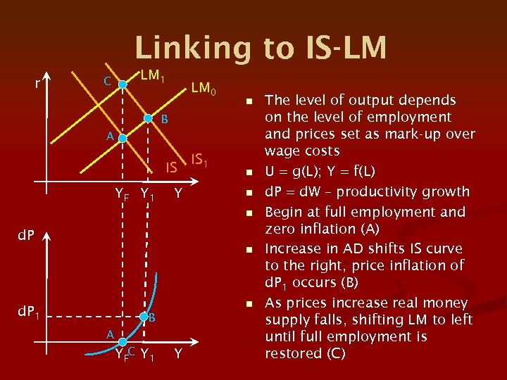Linking to IS-LM r C LM 1 LM 0 n B A IS YF Y 1 Y IS 1 n n n d. P 1 B A YFC Y 1 Y The level of output depends on the level of employment and prices set as mark-up over wage costs U = g(L); Y = f(L) d. P = d. W – productivity growth Begin at full employment and zero inflation (A) Increase in AD shifts IS curve to the right, price inflation of d. P 1 occurs (B) As prices increase real money supply falls, shifting LM to left until full employment is restored (C)

Orthodox Keynesianism Central Propositions

n n First Proposition: Modern capitalism subject to periodic recessions caused by deficiency of aggregate demand. Recessions are undesirable departures from full employment. Second Proposition: The economy can be in one of two situations – a demand -constrained Keynesian regime or a full -employment supply-constrained classical regime.

n n n Third Proposition: Unemployment of labor is a major feature of a Keynesian regime and unemployment is involuntary. Fourth Proposition: Deviations from full employment need to be corrected, can be corrected and therefore should be corrected. Fifth Proposition: In modern capitalism, wages and prices are not perfectly flexible; changes in AD will have real effects on output and employment.

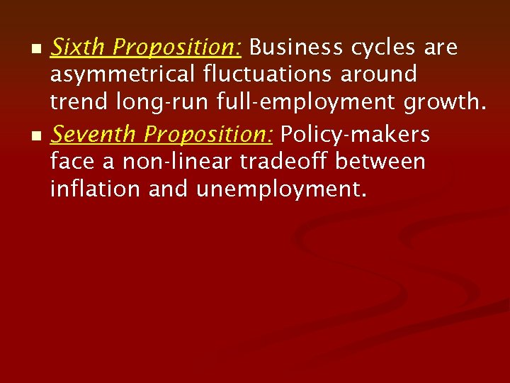n n Sixth Proposition: Business cycles are asymmetrical fluctuations around trend long-run full-employment growth. Seventh Proposition: Policy-makers face a non-linear tradeoff between inflation and unemployment.

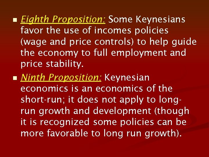n n Eighth Proposition: Some Keynesians favor the use of incomes policies (wage and price controls) to help guide the economy to full employment and price stability. Ninth Proposition: Keynesian economics is an economics of the short-run; it does not apply to longrun growth and development (though it is recognized some policies can be more favorable to long run growth).

Algebraic Summary of Basic IS-LM Model

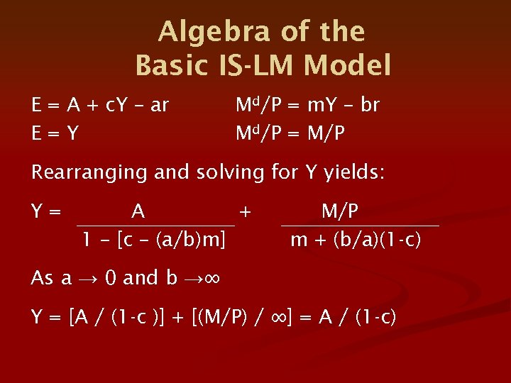Algebra of the Basic IS-LM Model E = A + c. Y – ar E=Y Md/P = m. Y – br Md/P = M/P Rearranging and solving for Y yields: Y= A + 1 – [c – (a/b)m] M/P m + (b/a)(1 -c) As a → 0 and b →∞ Y = [A / (1 -c )] + [(M/P) / ∞] = A / (1 -c)

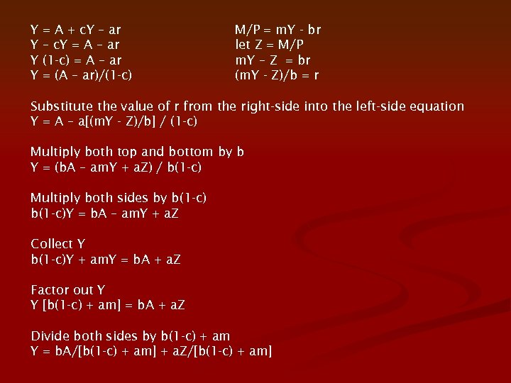Y Y = A + c. Y – ar – c. Y = A – ar (1 -c) = A – ar = (A – ar)/(1 -c) M/P = m. Y - br let Z = M/P m. Y – Z = br (m. Y - Z)/b = r Substitute the value of r from the right-side into the left-side equation Y = A – a[(m. Y - Z)/b] / (1 -c) Multiply both top and bottom by b Y = (b. A – am. Y + a. Z) / b(1 -c) Multiply both sides by b(1 -c)Y = b. A – am. Y + a. Z Collect Y b(1 -c)Y + am. Y = b. A + a. Z Factor out Y Y [b(1 -c) + am] = b. A + a. Z Divide both sides by b(1 -c) + am Y = b. A/[b(1 -c) + am] + a. Z/[b(1 -c) + am]

Y = b. A/[b(1 -c) + am] + a. Z/[b(1 -c) + am] Factor out b from 1 st term on right and factor out a from 2 nd term on right Y = {b. A/b[(1 – c) + (a/b)m]} + {a. Z/a[(b/a)(1 -c) + m] Cancel Y = A/[(1 – c) + (a/b)m] + Z/[(b/a)(1 -c) + m] Rearrange Y = A/[1 – (c – (a/b)m] + Z/[m + (b/a)(1 -c)] Replace Z with M/P Y= A 1 – [c – (a/b)m] + M/P m + (b/a)(1 -c)