Optimizing for the serial processors Scaled speedup

Optimizing for the serial processors • Scaled speedup: operate near the memory boundary. • Memory systems on modern processors are complicated. • The performance of a simple program can depend on the details of the micro-architecture. • Today we will study matrix multiplication optimizations • An important kernel in some scientific problems • Closely related to other algorithms, e. g. , transitive closure on a graph using Floyd-Warshall (is there a path between arbitrary vertices) • Optimization ideas can be used in other problems • The best case for optimization payoffs • The most well-studied algorithm in high performance computing Slide sources: Kathy Yellick UCB and Larry Carter UCSD

Outline • • • Performance Modeling Matrix-Vector Multiply (Warmup) Matrix Multiply Cache Optimizations Bag of Tricks Research in Matrix Multiply

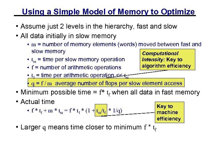Using a Simple Model of Memory to Optimize • Assume just 2 levels in the hierarchy, fast and slow • All data initially in slow memory • m = number of memory elements (words) moved between fast and slow memory Computational • tm = time per slow memory operation Intensity: Key to algorithm efficiency • f = number of arithmetic operations • tf = time per arithmetic operation << tm • q = f / m average number of flops per slow element access • Minimum possible time = f* tf when all data in fast memory • Actual time • f * tf + m * tm = f * tf * (1 + tm/tf * 1/q) • Larger q means time closer to minimum f * tf Key to machine efficiency

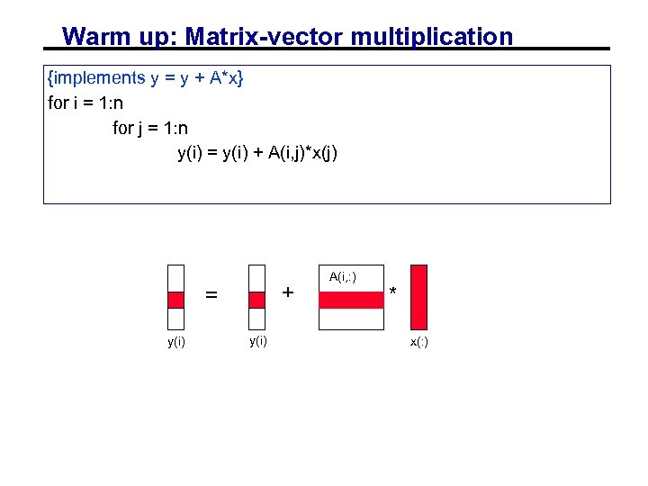Warm up: Matrix-vector multiplication {implements y = y + A*x} for i = 1: n for j = 1: n y(i) = y(i) + A(i, j)*x(j) + = y(i) A(i, : ) * x(: )

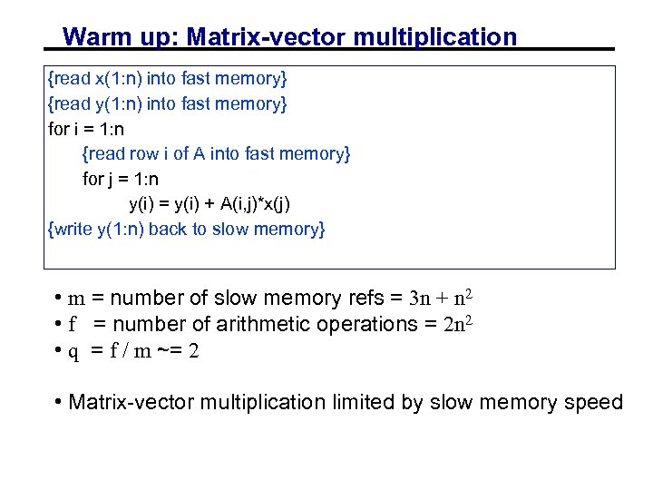Warm up: Matrix-vector multiplication {read x(1: n) into fast memory} {read y(1: n) into fast memory} for i = 1: n {read row i of A into fast memory} for j = 1: n y(i) = y(i) + A(i, j)*x(j) {write y(1: n) back to slow memory} • m = number of slow memory refs = 3 n + n 2 • f = number of arithmetic operations = 2 n 2 • q = f / m ~= 2 • Matrix-vector multiplication limited by slow memory speed

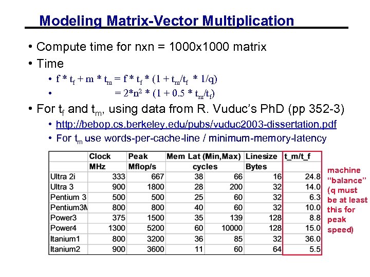Modeling Matrix-Vector Multiplication • Compute time for nxn = 1000 x 1000 matrix • Time • f * tf + m * tm = f * tf * (1 + tm/tf * 1/q) • = 2*n 2 * (1 + 0. 5 * tm/tf) • For tf and tm, using data from R. Vuduc’s Ph. D (pp 352 -3) • http: //bebop. cs. berkeley. edu/pubs/vuduc 2003 -dissertation. pdf • For tm use words-per-cache-line / minimum-memory-latency machine “balance” (q must be at least this for peak speed)

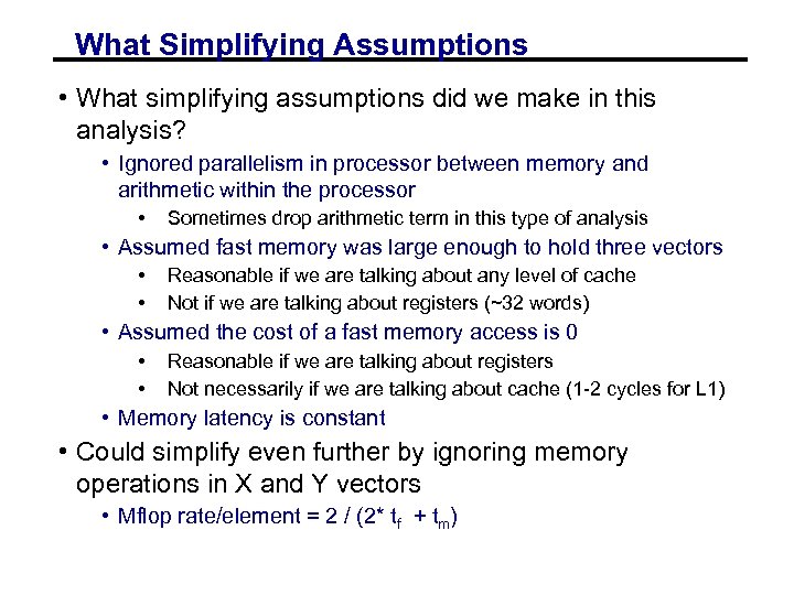What Simplifying Assumptions • What simplifying assumptions did we make in this analysis? • Ignored parallelism in processor between memory and arithmetic within the processor • Sometimes drop arithmetic term in this type of analysis • Assumed fast memory was large enough to hold three vectors • • Reasonable if we are talking about any level of cache Not if we are talking about registers (~32 words) • Assumed the cost of a fast memory access is 0 • • Reasonable if we are talking about registers Not necessarily if we are talking about cache (1 -2 cycles for L 1) • Memory latency is constant • Could simplify even further by ignoring memory operations in X and Y vectors • Mflop rate/element = 2 / (2* tf + tm)

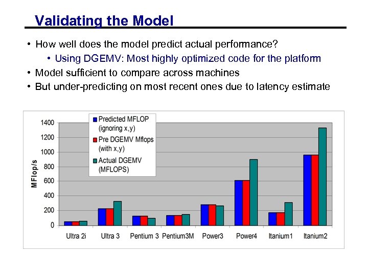Validating the Model • How well does the model predict actual performance? • Using DGEMV: Most highly optimized code for the platform • Model sufficient to compare across machines • But under-predicting on most recent ones due to latency estimate

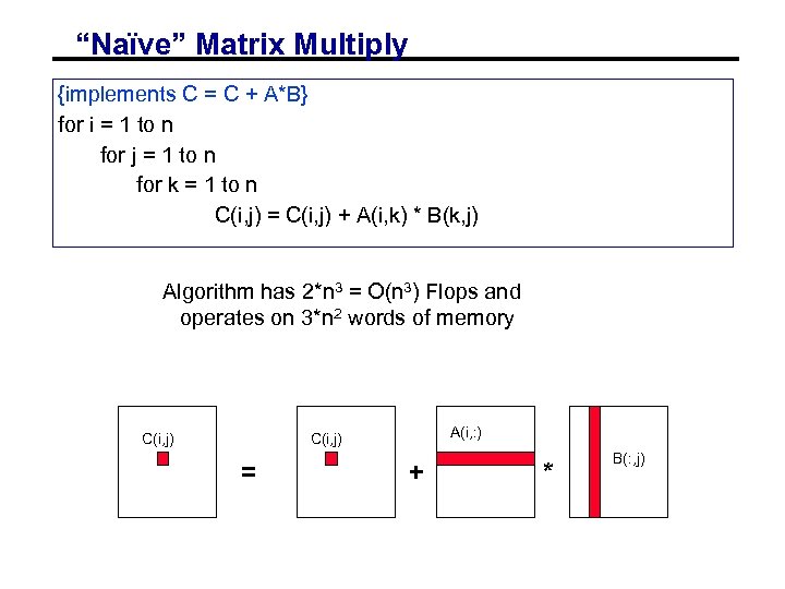“Naïve” Matrix Multiply {implements C = C + A*B} for i = 1 to n for j = 1 to n for k = 1 to n C(i, j) = C(i, j) + A(i, k) * B(k, j) Algorithm has 2*n 3 = O(n 3) Flops and operates on 3*n 2 words of memory C(i, j) A(i, : ) C(i, j) = + * B(: , j)

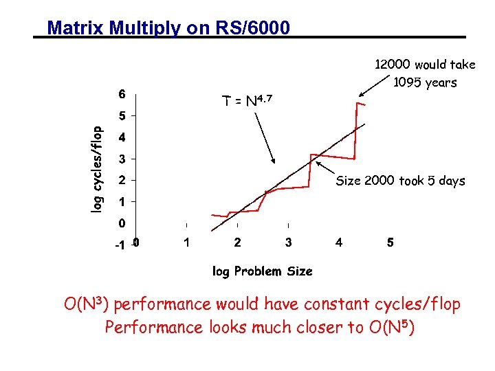Matrix Multiply on RS/6000 12000 would take 1095 years T = N 4. 7 Size 2000 took 5 days O(N 3) performance would have constant cycles/flop Performance looks much closer to O(N 5)

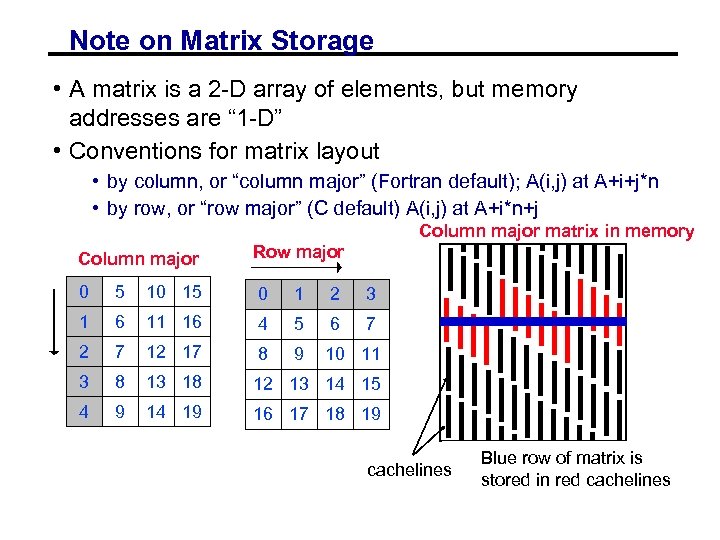Note on Matrix Storage • A matrix is a 2 -D array of elements, but memory addresses are “ 1 -D” • Conventions for matrix layout • by column, or “column major” (Fortran default); A(i, j) at A+i+j*n • by row, or “row major” (C default) A(i, j) at A+i*n+j Column major matrix in memory Column major Row major 0 5 10 15 0 1 2 3 1 6 11 16 4 5 6 7 2 7 12 17 8 9 10 11 3 8 13 18 12 13 14 15 4 9 14 19 16 17 18 19 cachelines Blue row of matrix is stored in red cachelines

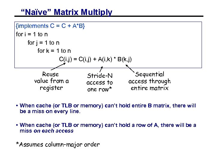“Naïve” Matrix Multiply {implements C = C + A*B} for i = 1 to n for j = 1 to n for k = 1 to n C(i, j) = C(i, j) + A(i, k) * B(k, j) Reuse value from a register Stride-N access to one row* Sequential access through entire matrix • When cache (or TLB or memory) can’t hold entire B matrix, there will be a miss on every line. • When cache (or TLB or memory) can’t hold a row of A, there will be a miss on each access *Assumes column-major order

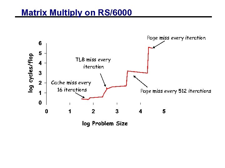Matrix Multiply on RS/6000 Page miss every iteration TLB miss every iteration Cache miss every 16 iterations Page miss every 512 iterations

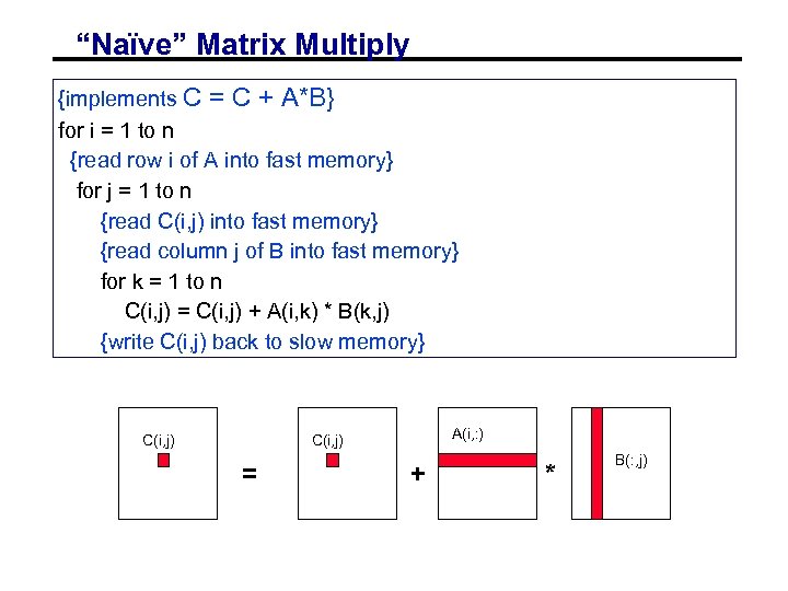“Naïve” Matrix Multiply {implements C = C + A*B} for i = 1 to n {read row i of A into fast memory} for j = 1 to n {read C(i, j) into fast memory} {read column j of B into fast memory} for k = 1 to n C(i, j) = C(i, j) + A(i, k) * B(k, j) {write C(i, j) back to slow memory} C(i, j) A(i, : ) C(i, j) = + * B(: , j)

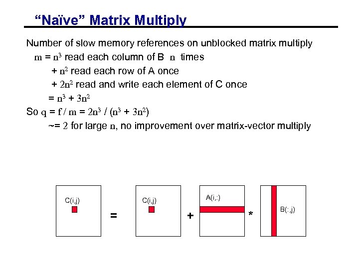“Naïve” Matrix Multiply Number of slow memory references on unblocked matrix multiply m = n 3 read each column of B n times + n 2 read each row of A once + 2 n 2 read and write each element of C once = n 3 + 3 n 2 So q = f / m = 2 n 3 / (n 3 + 3 n 2) ~= 2 for large n, no improvement over matrix-vector multiply C(i, j) A(i, : ) C(i, j) = + * B(: , j)

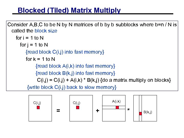Blocked (Tiled) Matrix Multiply Consider A, B, C to be N by N matrices of b by b subblocks where b=n / N is called the block size for i = 1 to N for j = 1 to N {read block C(i, j) into fast memory} for k = 1 to N {read block A(i, k) into fast memory} {read block B(k, j) into fast memory} C(i, j) = C(i, j) + A(i, k) * B(k, j) {do a matrix multiply on blocks} {write block C(i, j) back to slow memory} C(i, j) A(i, k) C(i, j) = + * B(k, j)

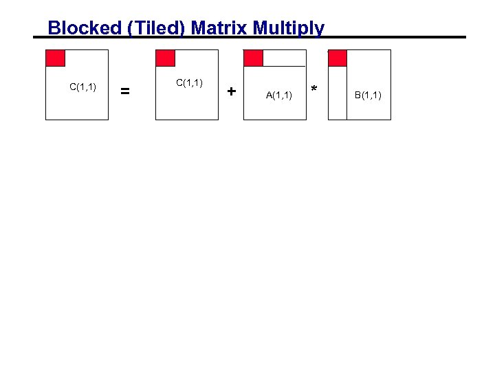Blocked (Tiled) Matrix Multiply C(1, 1) = C(1, 1) + A(1, 1) * B(1, 1)

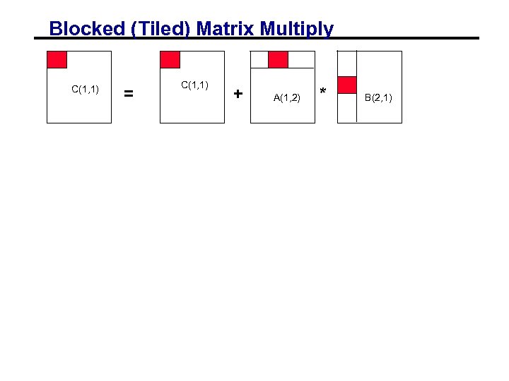Blocked (Tiled) Matrix Multiply C(1, 1) = C(1, 1) + A(1, 2) * B(2, 1)

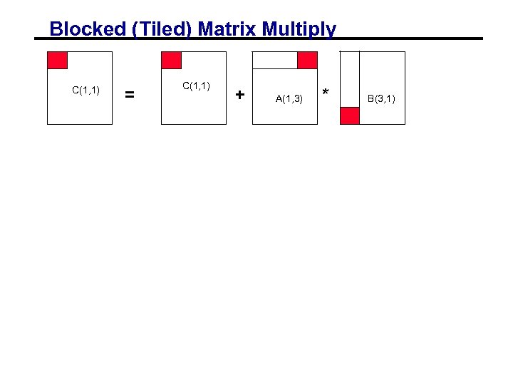Blocked (Tiled) Matrix Multiply C(1, 1) = C(1, 1) + A(1, 3) * B(3, 1)

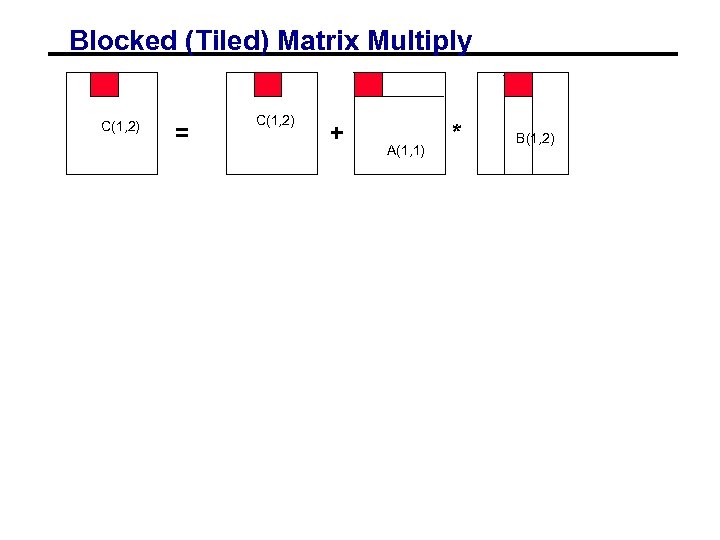Blocked (Tiled) Matrix Multiply C(1, 2) = C(1, 2) + A(1, 1) * B(1, 2)

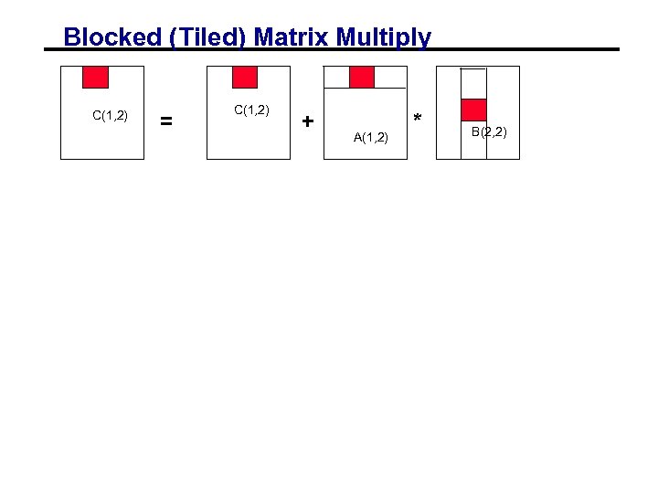Blocked (Tiled) Matrix Multiply C(1, 2) = C(1, 2) + A(1, 2) * B(2, 2)

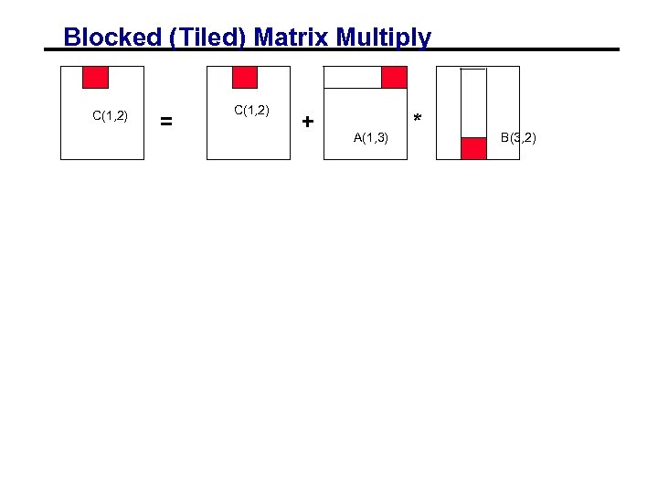Blocked (Tiled) Matrix Multiply C(1, 2) = C(1, 2) + A(1, 3) * B(3, 2)

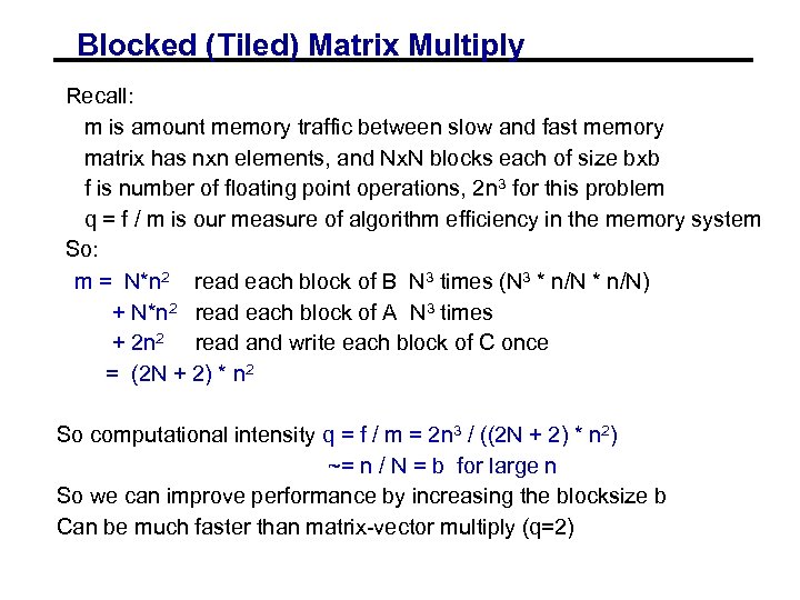Blocked (Tiled) Matrix Multiply Recall: m is amount memory traffic between slow and fast memory matrix has nxn elements, and Nx. N blocks each of size bxb f is number of floating point operations, 2 n 3 for this problem q = f / m is our measure of algorithm efficiency in the memory system So: m = N*n 2 read each block of B N 3 times (N 3 * n/N) + N*n 2 read each block of A N 3 times + 2 n 2 read and write each block of C once = (2 N + 2) * n 2 So computational intensity q = f / m = 2 n 3 / ((2 N + 2) * n 2) ~= n / N = b for large n So we can improve performance by increasing the blocksize b Can be much faster than matrix-vector multiply (q=2)

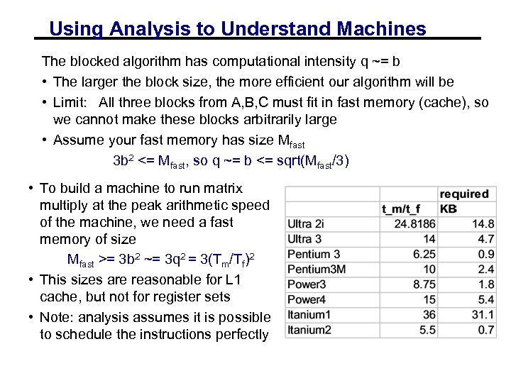Using Analysis to Understand Machines The blocked algorithm has computational intensity q ~= b • The larger the block size, the more efficient our algorithm will be • Limit: All three blocks from A, B, C must fit in fast memory (cache), so we cannot make these blocks arbitrarily large • Assume your fast memory has size Mfast 3 b 2 <= Mfast, so q ~= b <= sqrt(Mfast/3) • To build a machine to run matrix multiply at the peak arithmetic speed of the machine, we need a fast memory of size Mfast >= 3 b 2 ~= 3 q 2 = 3(Tm/Tf)2 • This sizes are reasonable for L 1 cache, but not for register sets • Note: analysis assumes it is possible to schedule the instructions perfectly

Limits to Optimizing Matrix Multiply • The blocked algorithm changes the order in which values are accumulated into each C[i, j] by applying associativity • The previous analysis showed that the blocked algorithm has computational intensity: q ~= b <= sqrt(Mfast/3) • There is a lower bound result that says we cannot do any better than this (using only algebraic associativity) • Theorem (Hong & Kung, 1981): Any reorganization of this algorithm (that uses only algebraic associativity) is limited to q = O(sqrt(Mfast))

Basic Linear Algebra Subroutines • Industry standard interface (evolving) • Vendors, others supply optimized implementations • History • BLAS 1 (1970 s): • • vector operations: dot product, saxpy (y=a*x+y), etc m=2*n, f=2*n, q ~1 or less • BLAS 2 (mid 1980 s) • • • matrix-vector operations: matrix vector multiply, etc m=n^2, f=2*n^2, q~2, less overhead somewhat faster than BLAS 1 • BLAS 3 (late 1980 s) • • matrix-matrix operations: matrix multiply, etc m >= 4 n^2, f=O(n^3), so q can possibly be as large as n, so BLAS 3 is potentially much faster than BLAS 2 • Good algorithms used BLAS 3 when possible (LAPACK) • See www. netlib. org/blas, www. netlib. org/lapack

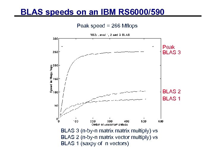BLAS speeds on an IBM RS 6000/590 Peak speed = 266 Mflops Peak BLAS 3 BLAS 2 BLAS 1 BLAS 3 (n-by-n matrix multiply) vs BLAS 2 (n-by-n matrix vector multiply) vs BLAS 1 (saxpy of n vectors)

Search Over Block Sizes • Performance models are useful for high level algorithms • Helps in developing a blocked algorithm • Models have not proven very useful for block size selection • • too complicated to be useful – See work by Sid Chatterjee for detailed model too simple to be accurate – Multiple multidimensional arrays, virtual memory, etc. • Some systems use search • Atlas – being incorporated into Matlab • Be. BOP – http: //www. cs. berkeley. edu/~richie/bebop

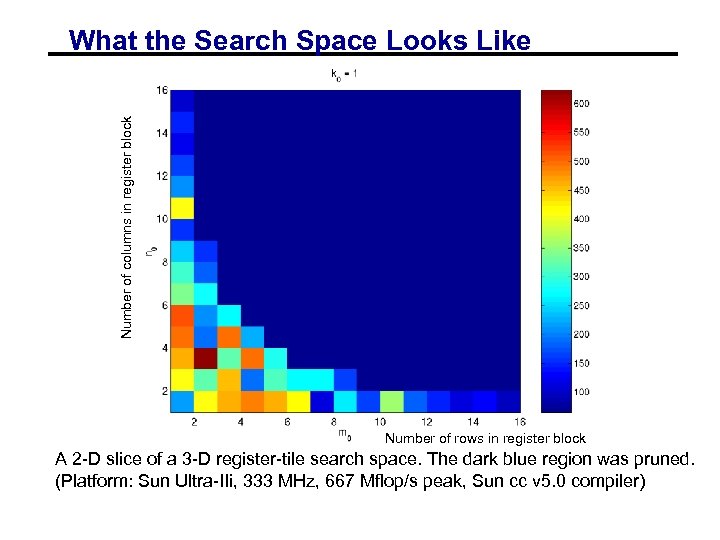Number of columns in register block What the Search Space Looks Like Number of rows in register block A 2 -D slice of a 3 -D register-tile search space. The dark blue region was pruned. (Platform: Sun Ultra-IIi, 333 MHz, 667 Mflop/s peak, Sun cc v 5. 0 compiler)

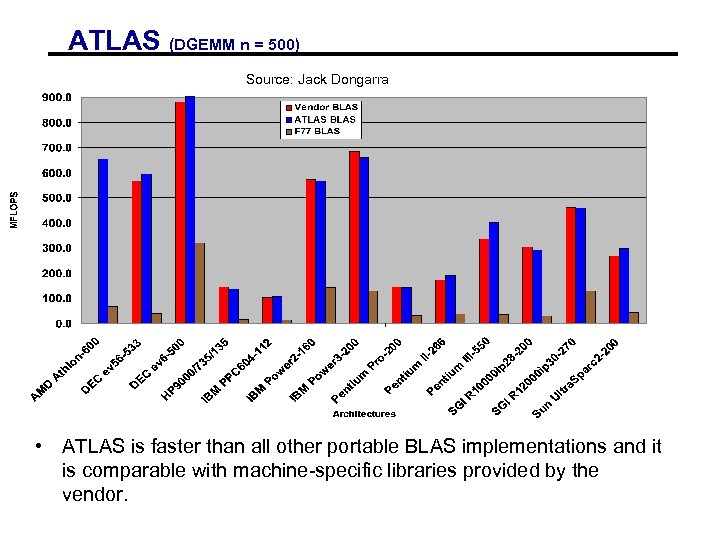ATLAS (DGEMM n = 500) Source: Jack Dongarra • ATLAS is faster than all other portable BLAS implementations and it is comparable with machine-specific libraries provided by the vendor.

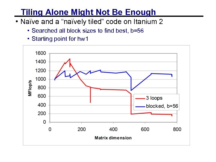Tiling Alone Might Not Be Enough • Naïve and a “naïvely tiled” code on Itanium 2 • Searched all block sizes to find best, b=56 • Starting point for hw 1

Optimizing in Practice • Tiling for registers • loop unrolling, use of named “register” variables • Tiling for multiple levels of cache and TLB • Exploiting fine-grained parallelism in processor • superscalar; pipelining • Complicated compiler interactions • Hard to do by hand (but you’ll try) • Automatic optimization an active research area • Be. BOP: bebop. cs. berkeley. edu/ • PHi. PAC: www. icsi. berkeley. edu/~bilmes/phipac in particular tr-98 -035. ps. gz • ATLAS: www. netlib. org/atlas

Removing False Dependencies • Using local variables, reorder operations to remove false dependencies a[i] = b[i] + c; a[i+1] = b[i+1] * d; false read-after-write hazard between a[i] and b[i+1] float f 1 = b[i]; float f 2 = b[i+1]; a[i] = f 1 + c; a[i+1] = f 2 * d; With some compilers, you can declare a and b unaliased. • Done via “restrict pointers, ” compiler flag, or pragma)

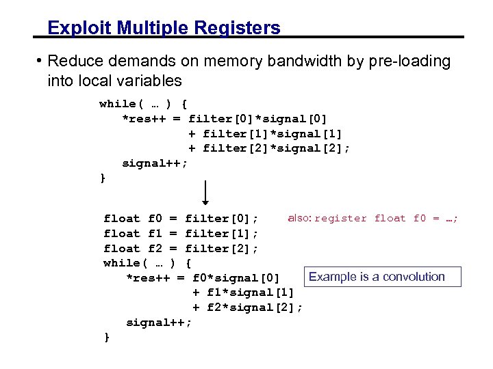Exploit Multiple Registers • Reduce demands on memory bandwidth by pre-loading into local variables while( … ) { *res++ = filter[0]*signal[0] + filter[1]*signal[1] + filter[2]*signal[2]; signal++; } also: register float f 0 = …; float f 0 = filter[0]; float f 1 = filter[1]; float f 2 = filter[2]; while( … ) { Example is a convolution *res++ = f 0*signal[0] + f 1*signal[1] + f 2*signal[2]; signal++; }

Loop Unrolling • Expose instruction-level parallelism float f 0 = filter[0], f 1 = filter[1], f 2 = filter[2]; float s 0 = signal[0], s 1 = signal[1], s 2 = signal[2]; *res++ = f 0*s 0 + f 1*s 1 + f 2*s 2; do { signal += 3; s 0 = signal[0]; res[0] = f 0*s 1 + f 1*s 2 + f 2*s 0; s 1 = signal[1]; res[1] = f 0*s 2 + f 1*s 0 + f 2*s 1; s 2 = signal[2]; res[2] = f 0*s 0 + f 1*s 1 + f 2*s 2; res += 3; } while( … );

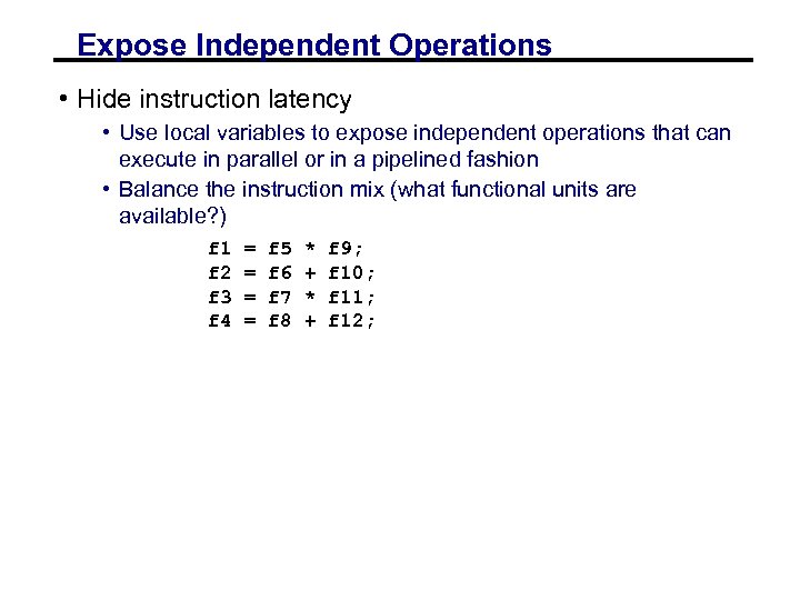Expose Independent Operations • Hide instruction latency • Use local variables to expose independent operations that can execute in parallel or in a pipelined fashion • Balance the instruction mix (what functional units are available? ) f 1 f 2 f 3 f 4 = = f 5 f 6 f 7 f 8 * + f 9; f 10; f 11; f 12;

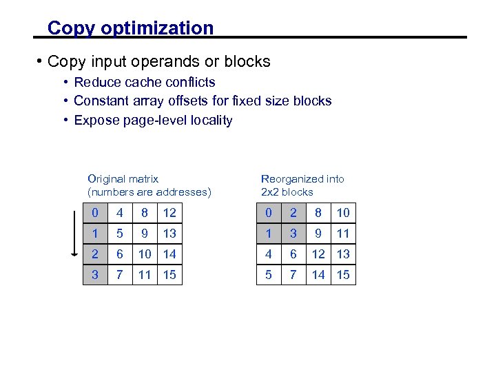Copy optimization • Copy input operands or blocks • Reduce cache conflicts • Constant array offsets for fixed size blocks • Expose page-level locality Original matrix (numbers are addresses) Reorganized into 2 x 2 blocks 0 4 8 12 0 2 8 10 1 5 9 13 1 3 9 11 2 6 10 14 4 6 12 13 3 7 11 15 5 7 14 15

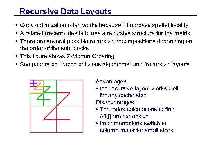Recursive Data Layouts • Copy optimization often works because it improves spatial locality • A related (recent) idea is to use a recursive structure for the matrix • There are several possible recursive decompositions depending on the order of the sub-blocks • This figure shows Z-Morton Ordering • See papers on “cache oblivious algorithms” and “recursive layouts” Advantages: • the recursive layout works well for any cache size Disadvantages: • The index calculations to find A[i, j] are expensive • Implementations switch to column-major for small sizes

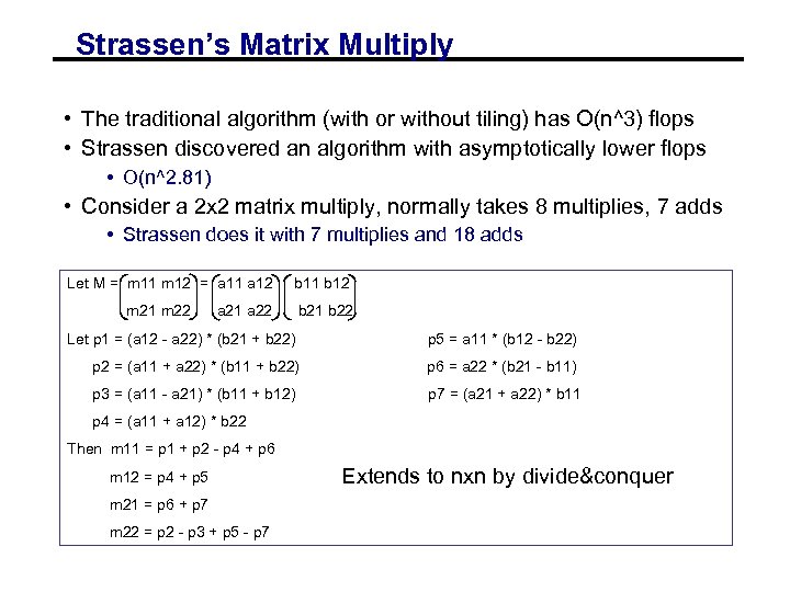Strassen’s Matrix Multiply • The traditional algorithm (with or without tiling) has O(n^3) flops • Strassen discovered an algorithm with asymptotically lower flops • O(n^2. 81) • Consider a 2 x 2 matrix multiply, normally takes 8 multiplies, 7 adds • Strassen does it with 7 multiplies and 18 adds Let M = m 11 m 12 = a 11 a 12 b 11 b 12 m 21 m 22 = a 21 a 22 b 21 b 22 Let p 1 = (a 12 - a 22) * (b 21 + b 22) p 5 = a 11 * (b 12 - b 22) p 2 = (a 11 + a 22) * (b 11 + b 22) p 6 = a 22 * (b 21 - b 11) p 3 = (a 11 - a 21) * (b 11 + b 12) p 7 = (a 21 + a 22) * b 11 p 4 = (a 11 + a 12) * b 22 Then m 11 = p 1 + p 2 - p 4 + p 6 m 12 = p 4 + p 5 m 21 = p 6 + p 7 m 22 = p 2 - p 3 + p 5 - p 7 Extends to nxn by divide&conquer

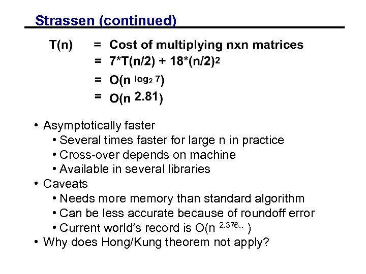Strassen (continued) • Asymptotically faster • Several times faster for large n in practice • Cross-over depends on machine • Available in several libraries • Caveats • Needs more memory than standard algorithm • Can be less accurate because of roundoff error • Current world’s record is O(n 2. 376. . ) • Why does Hong/Kung theorem not apply?

Locality in Other Algorithms • The performance of any algorithm is limited by q • In matrix multiply, we increase q by changing computation order • increased temporal locality • For other algorithms and data structures, even handtransformations are still an open problem • sparse matrices (reordering, blocking) • trees (B-Trees are for the disk level of the hierarchy) • linked lists (some work done here)

Summary • Performance programming on uniprocessors requires • understanding of memory system • understanding of fine-grained parallelism in processor • Simple performance models can aid in understanding • Two ratios are key to efficiency (relative to peak) 1. computational intensity of the algorithm: • q = f/m = # floating point opns / # slow memory opns 2. machine balance in the memory system: • tm/tf = time for slow memory operation / time for floating point operation • Blocking (tiling) is a basic approach • Techniques apply generally, but the details (e. g. , block size) are architecture dependent • Similar techniques are possible on other data structures and algorithms

Reading • "Performance Optimization of Numerically Intensive Codes", by Stefan Goedecker and Adolfy Hoisie, SIAM 2001. • Web pages for reference: • Be. BOP Homepage • ATLAS Homepage • BLAS (Basic Linear Algebra Subroutines), Reference for (unoptimized) implementations of the BLAS, with documentation. • LAPACK (Linear Algebra PACKage), a standard linear algebra library optimized to use the BLAS effectively on uniprocessors and shared memory machines (software, documentation and reports) • Sca. LAPACK (Scalable LAPACK), a parallel version of LAPACK for distributed memory machines (software, documentation and reports) • Tuning Strassen's Matrix Multiplication for Memory Efficiency Mithuna S. Thottethodi, Siddhartha Chatterjee, and Alvin R. Lebeck in Proceedings of Supercomputing '98, November 1998 postscript • Recursive Array Layouts and Fast Parallel Matrix Multiplication” by Chatterjee et al. IEEE TPDS November 2002.

Questions You Should Be Able to Answer 1. What is the key to understand algorithm efficiency in our simple memory model? 2. What is the key to understand machine efficiency in our simple memory model? 3. What is tiling? 4. Why does block matrix multiply reduce the number of memory references? 5. What are the BLAS? 6. What is LAPACK? Sca. LAPACK? 7. Why does loop unrolling improve uniprocessor performance?

Review from Last Lecture 08/29/2002 CS 267 Lecure 2 46

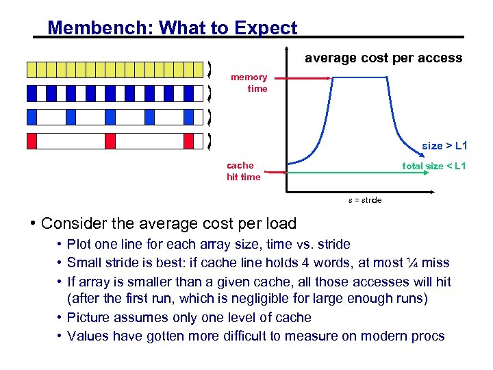Membench: What to Expect average cost per access memory time size > L 1 cache hit time total size < L 1 s = stride • Consider the average cost per load • Plot one line for each array size, time vs. stride • Small stride is best: if cache line holds 4 words, at most ¼ miss • If array is smaller than a given cache, all those accesses will hit (after the first run, which is negligible for large enough runs) • Picture assumes only one level of cache • Values have gotten more difficult to measure on modern procs

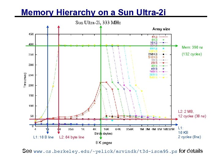Memory Hierarchy on a Sun Ultra-2 i, 333 MHz Array size Mem: 396 ns (132 cycles) L 2: 2 MB, 12 cycles (36 ns) L 1: 16 B line L 1: 16 KB 2 cycles (6 ns) L 2: 64 byte line 8 K pages See www. cs. berkeley. edu/~yelick/arvindk/t 3 d-isca 95. ps for details

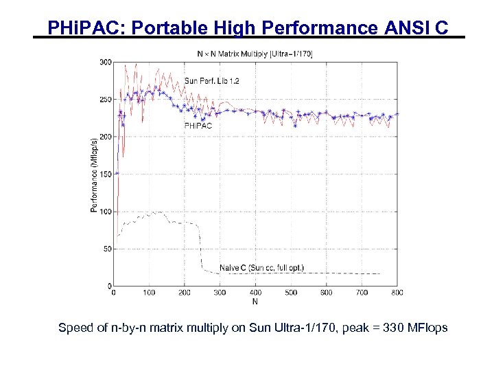PHi. PAC: Portable High Performance ANSI C Speed of n-by-n matrix multiply on Sun Ultra-1/170, peak = 330 MFlops