22697f9f95b7986ae2d53c78fea2be9c.ppt
- Количество слайдов: 49
 Operations Management Module D – Waiting-Line Models Power. Point presentation to accompany Heizer/Render Principles of Operations Management, 7 e Operations Management, 9 e © 2008 Prentice Hall, Inc. D–
 Outline þ Characteristics of a Waiting-Line System þ Arrival Characteristics þ Waiting-Line Characteristics þ Service Characteristics þ Measuring a Queue’s Performance þ Queuing Costs © 2008 Prentice Hall, Inc. D– 2
 Outline – Continued þ The Variety of Queuing Models þ Model A(M/M/1): Single-Channel Queuing Model with Poisson Arrivals and Exponential Service Times þ Model B(M/M/S): Multiple-Channel Queuing Model þ Model C(M/D/1): Constant-Service-Time Model þ Model D: Limited-Population Model © 2008 Prentice Hall, Inc. D– 3
 Outline – Continued þ Other Queuing Approaches © 2008 Prentice Hall, Inc. D– 4
 Learning Objectives When you complete this module you should be able to: 1. Describe the characteristics of arrivals, waiting lines, and service systems 2. Apply the single-channel queuing model equations 3. Conduct a cost analysis for a waiting line © 2008 Prentice Hall, Inc. D– 5
 Learning Objectives When you complete this module you should be able to: 4. Apply the multiple-channel queuing model formulas 5. Apply the constant-service-time model equations 6. Perform a limited-population model analysis © 2008 Prentice Hall, Inc. D– 6
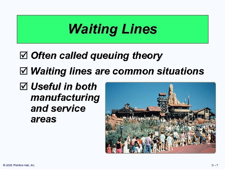 Waiting Lines þ Often called queuing theory þ Waiting lines are common situations þ Useful in both manufacturing and service areas © 2008 Prentice Hall, Inc. D– 7
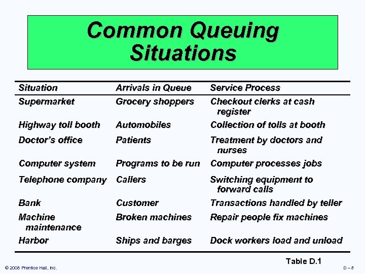 Common Queuing Situations Situation Supermarket Arrivals in Queue Grocery shoppers Highway toll booth Automobiles Doctor’s office Patients Computer system Programs to be run Telephone company Callers Service Process Checkout clerks at cash register Collection of tolls at booth Treatment by doctors and nurses Computer processes jobs Bank Customer Switching equipment to forward calls Transactions handled by teller Machine maintenance Harbor Broken machines Repair people fix machines Ships and barges Dock workers load and unload © 2008 Prentice Hall, Inc. Table D. 1 D– 8
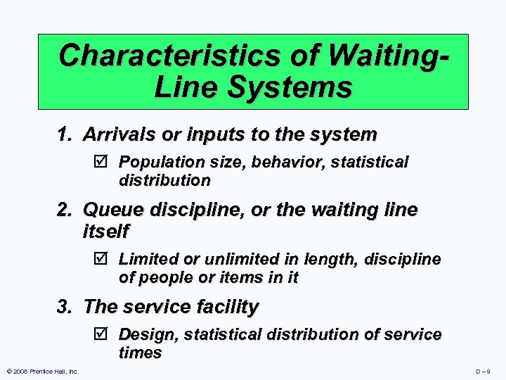 Characteristics of Waiting. Line Systems 1. Arrivals or inputs to the system þ Population size, behavior, statistical distribution 2. Queue discipline, or the waiting line itself þ Limited or unlimited in length, discipline of people or items in it 3. The service facility þ Design, statistical distribution of service times © 2008 Prentice Hall, Inc. D– 9
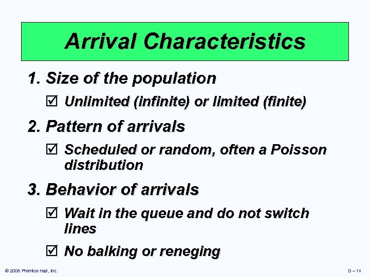 Arrival Characteristics 1. Size of the population þ Unlimited (infinite) or limited (finite) 2. Pattern of arrivals þ Scheduled or random, often a Poisson distribution 3. Behavior of arrivals þ Wait in the queue and do not switch lines þ No balking or reneging © 2008 Prentice Hall, Inc. D – 10
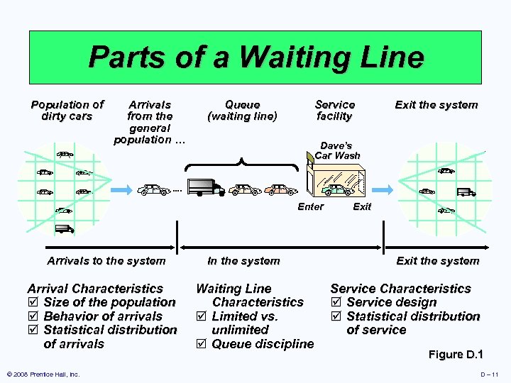 Parts of a Waiting Line Population of dirty cars Arrivals from the general population … Queue (waiting line) Service facility Dave’s Car Wash Enter Arrivals to the system Arrival Characteristics þ Size of the population þ Behavior of arrivals þ Statistical distribution of arrivals © 2008 Prentice Hall, Inc. Exit the system In the system Waiting Line Characteristics þ Limited vs. unlimited þ Queue discipline Exit the system Service Characteristics þ Service design þ Statistical distribution of service Figure D. 1 D – 11
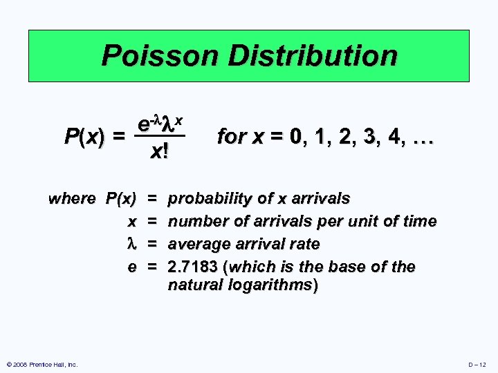 Poisson Distribution e - x P (x ) = x! where P(x) x e © 2008 Prentice Hall, Inc. = = for x = 0, 1, 2, 3, 4, … probability of x arrivals number of arrivals per unit of time average arrival rate 2. 7183 (which is the base of the natural logarithms) D – 12
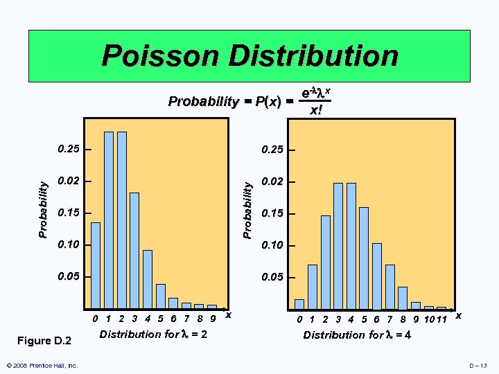 Poisson Distribution e- x Probability = P(x) = x! 0. 25 – 0. 02 – Probability 0. 25 – 0. 10 – 0. 05 – – Figure D. 2 © 2008 Prentice Hall, Inc. 0. 15 – 0. 10 – 0. 05 – 0 1 2 3 4 5 6 7 8 9 x Distribution for = 2 – 0 1 2 3 4 5 6 7 8 9 10 11 x Distribution for = 4 D – 13
 Waiting-Line Characteristics þ Limited or unlimited queue length þ Queue discipline - first-in, first-out (FIFO) is most common þ Other priority rules may be used in special circumstances © 2008 Prentice Hall, Inc. D – 14
 Service Characteristics þ Queuing system designs þ Single-channel system, multiplechannel system þ Single-phase system, multiphase system þ Service time distribution þ Constant service time þ Random service times, usually a negative exponential distribution © 2008 Prentice Hall, Inc. D – 15
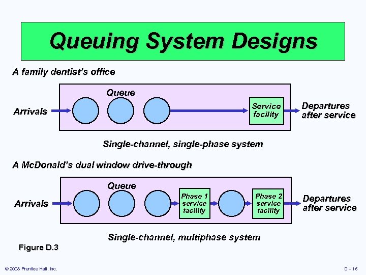 Queuing System Designs A family dentist’s office Queue Service facility Arrivals Departures after service Single-channel, single-phase system A Mc. Donald’s dual window drive-through Queue Arrivals Phase 1 service facility Phase 2 service facility Departures after service Single-channel, multiphase system Figure D. 3 © 2008 Prentice Hall, Inc. D – 16
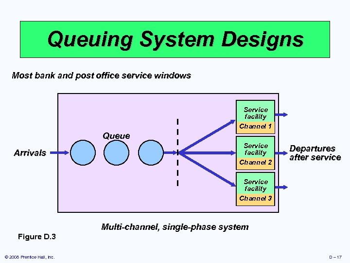 Queuing System Designs Most bank and post office service windows Service facility Channel 1 Queue Arrivals Service facility Channel 2 Departures after service Service facility Channel 3 Multi-channel, single-phase system Figure D. 3 © 2008 Prentice Hall, Inc. D – 17
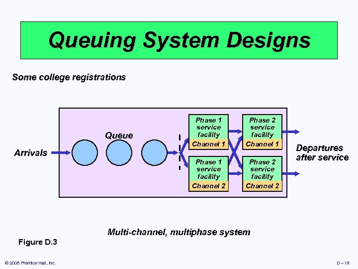 Queuing System Designs Some college registrations Arrivals Phase 2 service facility Channel 1 Phase 1 service facility Channel 2 Queue Phase 1 service facility Channel 1 Phase 2 service facility Channel 2 Departures after service Multi-channel, multiphase system Figure D. 3 © 2008 Prentice Hall, Inc. D – 18
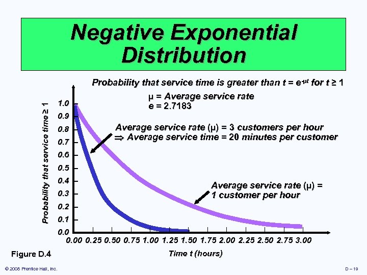 Probability that service time ≥ 1 Negative Exponential Distribution 1. 0 – 0. 9 – 0. 8 – 0. 7 – -µt Probability that service time is greater than t = e-µt for t ≥ 1 µ = Average service rate e = 2. 7183 Average service rate (µ) = 3 customers per hour Average service time = 20 minutes per customer 0. 6 – 0. 5 – 0. 4 – 0. 3 – Average service rate (µ) = 1 customer per hour 0. 2 – 0. 1 – | | | 0. 0 |– 0. 00 0. 25 0. 50 0. 75 1. 00 1. 25 1. 50 1. 75 2. 00 2. 25 2. 50 2. 75 3. 00 Figure D. 4 © 2008 Prentice Hall, Inc. Time t (hours) D – 19
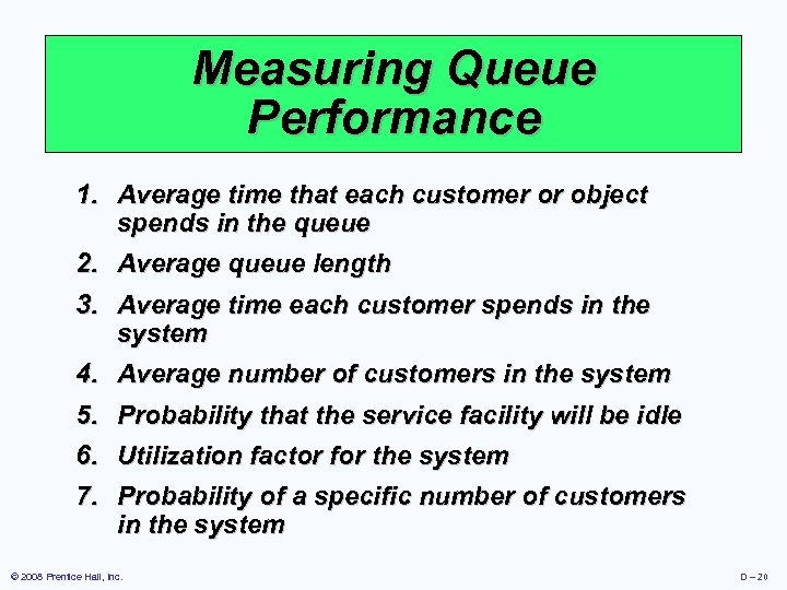 Measuring Queue Performance 1. Average time that each customer or object spends in the queue 2. Average queue length 3. Average time each customer spends in the system 4. Average number of customers in the system 5. Probability that the service facility will be idle 6. Utilization factor for the system 7. Probability of a specific number of customers in the system © 2008 Prentice Hall, Inc. D – 20
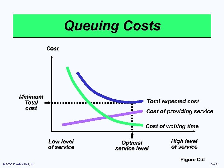 Queuing Costs Cost Minimum Total cost Total expected cost Cost of providing service Cost of waiting time Low level of service Optimal service level High level of service Figure D. 5 © 2008 Prentice Hall, Inc. D – 21
 Queuing Models The four queuing models here all assume: þ Poisson distribution arrivals þ FIFO discipline þ A single-service phase © 2008 Prentice Hall, Inc. D – 22
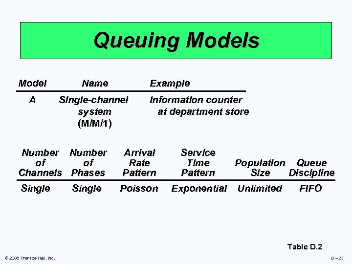 Queuing Models Model Name Example A Single-channel system (M/M/1) Information counter at department store Number of of Channels Phases Arrival Rate Pattern Service Time Pattern Single Poisson Exponential Single Population Queue Size Discipline Unlimited FIFO Table D. 2 © 2008 Prentice Hall, Inc. D – 23
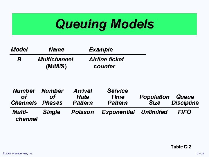 Queuing Models Model Name Example B Multichannel (M/M/S) Airline ticket counter Number of of Channels Phases Arrival Rate Pattern Service Time Pattern Multi. Single channel Poisson Exponential Population Queue Size Discipline Unlimited FIFO Table D. 2 © 2008 Prentice Hall, Inc. D – 24
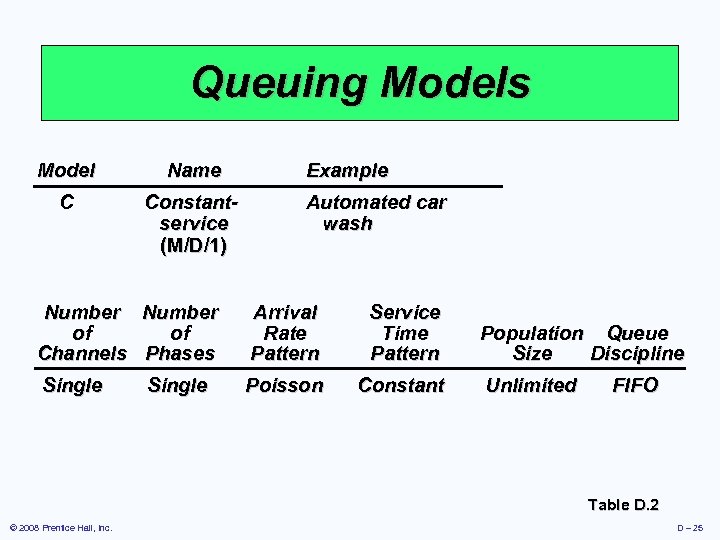 Queuing Models Model Name C Constantservice (M/D/1) Example Automated car wash Number of of Channels Phases Arrival Rate Pattern Service Time Pattern Single Poisson Constant Single Population Queue Size Discipline Unlimited FIFO Table D. 2 © 2008 Prentice Hall, Inc. D – 25
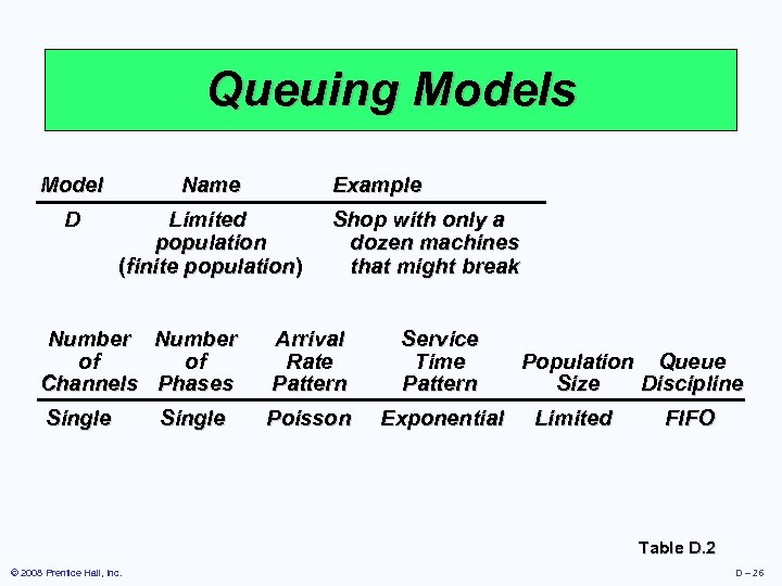 Queuing Models Model Name Example D Limited population (finite population) Shop with only a dozen machines that might break Number of of Channels Phases Arrival Rate Pattern Service Time Pattern Single Poisson Exponential Single Population Queue Size Discipline Limited FIFO Table D. 2 © 2008 Prentice Hall, Inc. D – 26
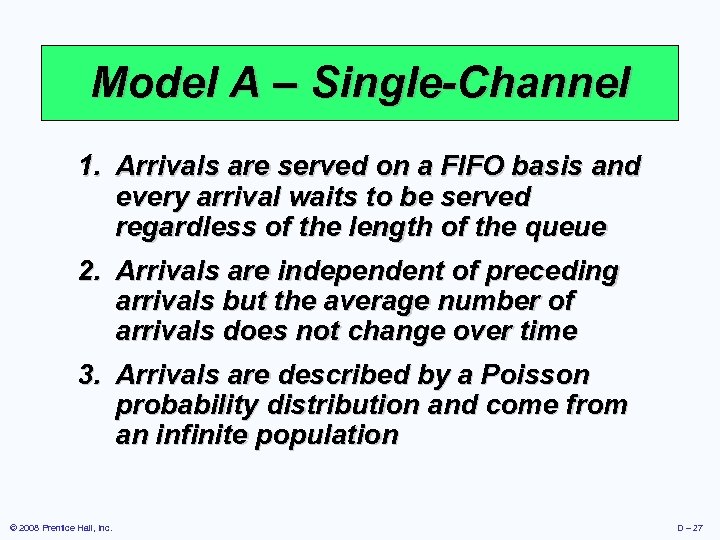 Model A – Single-Channel 1. Arrivals are served on a FIFO basis and every arrival waits to be served regardless of the length of the queue 2. Arrivals are independent of preceding arrivals but the average number of arrivals does not change over time 3. Arrivals are described by a Poisson probability distribution and come from an infinite population © 2008 Prentice Hall, Inc. D – 27
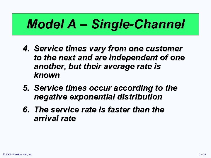 Model A – Single-Channel 4. Service times vary from one customer to the next and are independent of one another, but their average rate is known 5. Service times occur according to the negative exponential distribution 6. The service rate is faster than the arrival rate © 2008 Prentice Hall, Inc. D – 28
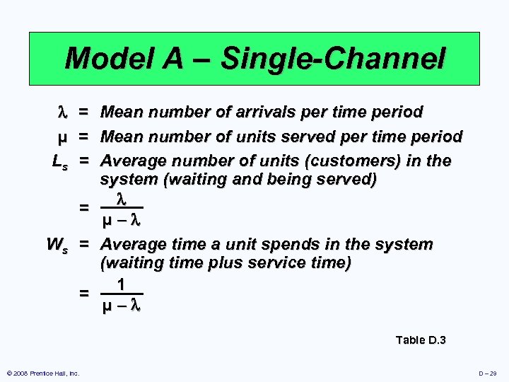 Model A – Single-Channel µ Ls = = = Mean number of arrivals per time period Mean number of units served per time period Average number of units (customers) in the system (waiting and being served) = µ– Ws = Average time a unit spends in the system (waiting time plus service time) 1 = µ– Table D. 3 © 2008 Prentice Hall, Inc. D – 29
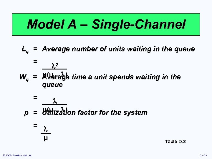 Model A – Single-Channel Lq = Average number of units waiting in the queue = 2 µ(µ – ) Wq = Average time a unit spends waiting in the queue = µ(µ – ) p = Utilization factor for the system = © 2008 Prentice Hall, Inc. µ Table D. 3 D – 30
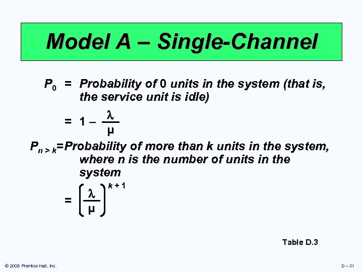 Model A – Single-Channel P 0 = Probability of 0 units in the system (that is, the service unit is idle) = 1– µ Pn > k= Probability of more than k units in the system, where n is the number of units in the system = µ k+1 Table D. 3 © 2008 Prentice Hall, Inc. D – 31
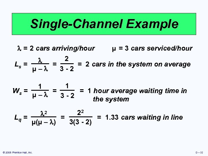 Single-Channel Example = 2 cars arriving/hour µ = 3 cars serviced/hour 2 Ls = = = 2 cars in the system on average 3 -2 µ– 1 1 Ws = = = 1 hour average waiting time in µ– 3 -2 the system 22 2 Lq = = = 1. 33 cars waiting in line 3(3 - 2) µ(µ – ) © 2008 Prentice Hall, Inc. D – 32
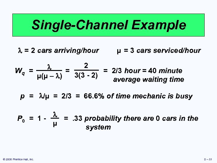 Single-Channel Example = 2 cars arriving/hour µ = 3 cars serviced/hour 2 Wq = = = 2/3 hour = 40 minute 3(3 - 2) µ(µ – ) average waiting time p = /µ = 2/3 = 66. 6% of time mechanic is busy P 0 = 1 =. 33 probability there are 0 cars in the µ system © 2008 Prentice Hall, Inc. D – 33
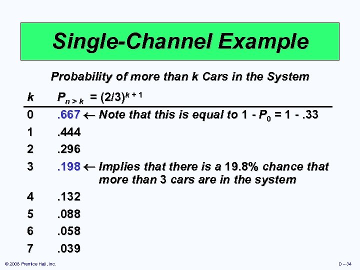 Single-Channel Example Probability of more than k Cars in the System k 0 1 2 3 4 5 6 7 © 2008 Prentice Hall, Inc. Pn > k = (2/3)k + 1. 667 Note that this is equal to 1 - P 0 = 1 -. 33. 444. 296. 198 Implies that there is a 19. 8% chance that more than 3 cars are in the system. 132. 088. 058. 039 D – 34
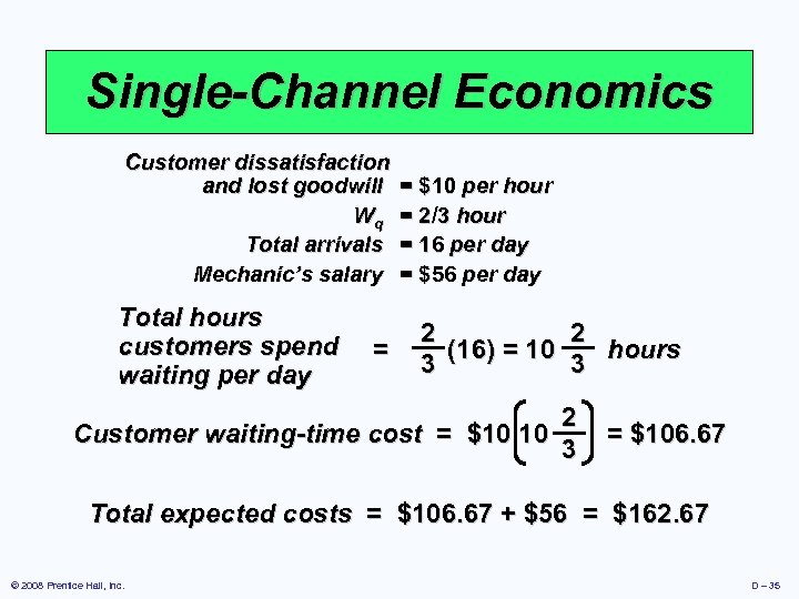 Single-Channel Economics Customer dissatisfaction and lost goodwill Wq Total arrivals Mechanic’s salary Total hours customers spend waiting per day = = $10 per hour = 2/3 hour = 16 per day = $56 per day 2 2 (16) = 10 hours 3 3 Customer waiting-time cost = $10 10 2 3 = $106. 67 Total expected costs = $106. 67 + $56 = $162. 67 © 2008 Prentice Hall, Inc. D – 35
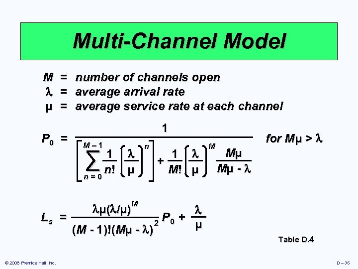 Multi-Channel Model M µ = = = P 0 = number of channels open average arrival rate average service rate at each channel 1 M– 1 ∑ 1 n! n=0 µ n 1 + M! µ M for M µ > Mµ Mµ - M µ( /µ) Ls = P + 2 0 µ (M - 1)!(Mµ - ) © 2008 Prentice Hall, Inc. Table D. 4 D – 36
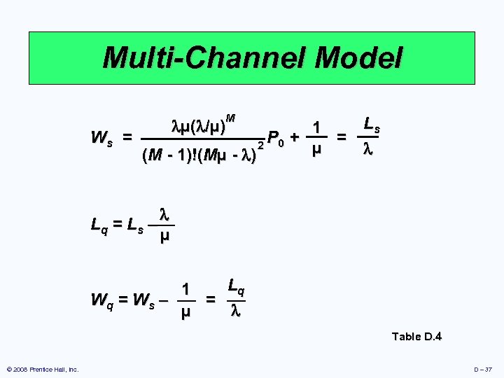 Multi-Channel Model M µ( /µ) 1 Ws = P + = 2 0 µ (M - 1)!(Mµ - ) Ls Lq = L s – µ Lq 1 Wq = W s – = µ Table D. 4 © 2008 Prentice Hall, Inc. D – 37
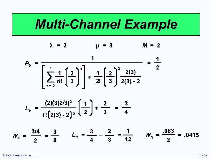 Multi-Channel Example = 2 P 0 = 1 n=0 Ws = 3/4 © 2008 Prentice Hall, Inc. 2 M = 2 1 ∑ Ls = µ = 3 1 n! 2 3 (2)(3(2/3)2 1! 2(3) - 2 3 = 8 2 n 1 + 2! 1 2 Lq = 2 + 3 2 2(3) 1 = 2 2(3) - 2 = 3 4 1 2 3 – = 12 3 4 Wq = . 083 2 =. 0415 D – 38
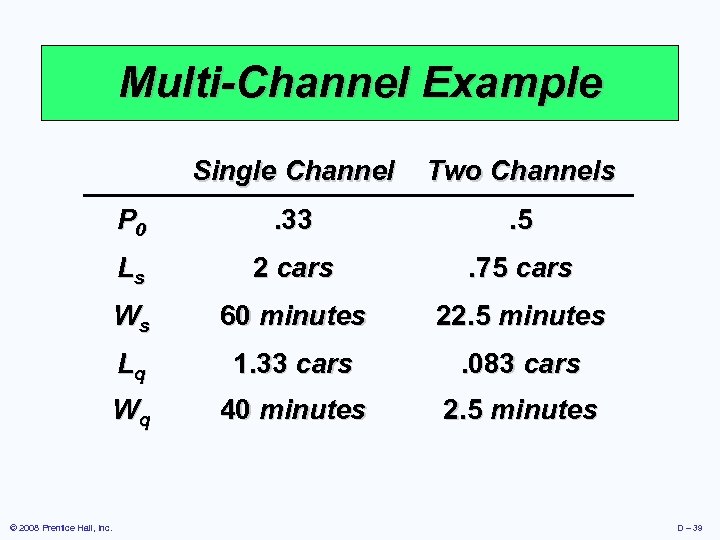 Multi-Channel Example Single Channel P 0 . 33 . 5 Ls 2 cars . 75 cars Ws 60 minutes 22. 5 minutes Lq 1. 33 cars . 083 cars Wq © 2008 Prentice Hall, Inc. Two Channels 40 minutes 2. 5 minutes D – 39
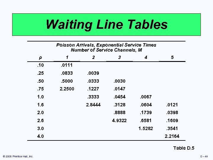 Waiting Line Tables ρ Poisson Arrivals, Exponential Service Times Number of Service Channels, M 1 2 3 4 5 . 10 . 0111 . 25 . 0833 . 0039 . 5000 . 0333 . 0030 . 75 2. 2500 . 1227 . 0147 1. 0 . 3333 . 0454 . 0067 1. 6 2. 8444 . 3128 . 0604 . 0121 2. 0 . 8888 . 1739 . 0398 2. 6 4. 9322 . 6581 . 1609 1. 5282 . 3541 3. 0 4. 0 2. 2164 Table D. 5 © 2008 Prentice Hall, Inc. D – 40
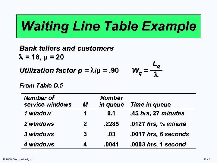 Waiting Line Table Example Bank tellers and customers = 18, µ = 20 Utilization factor ρ = /µ =. 90 Lq Wq = From Table D. 5 Number of service windows 1 window M 1 Number in queue 8. 1 Time in queue. 45 hrs, 27 minutes 2 windows 2 . 2285 . 0127 hrs, ¾ minute 3 windows 3 . 0017 hrs, 6 seconds 4 windows 4 . 0041 . 0003 hrs, 1 second © 2008 Prentice Hall, Inc. D – 41
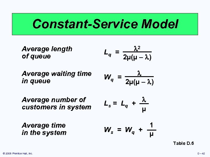 Constant-Service Model Average length of queue 2 Lq = 2µ(µ – ) Average waiting time in queue Wq = Average number of customers in system Ls = L q + µ Average time in the system 2µ(µ – ) Ws = W q + 1 µ Table D. 6 © 2008 Prentice Hall, Inc. D – 42
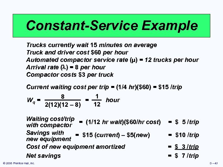 Constant-Service Example Trucks currently wait 15 minutes on average Truck and driver cost $60 per hour Automated compactor service rate (µ) = 12 trucks per hour Arrival rate ( ) = 8 per hour Compactor costs $3 per truck Current waiting cost per trip = (1/4 hr)($60) = $15 /trip 1 8 Wq = = hour 12 2(12)(12 – 8) Waiting cost/trip = (1/12 hr wait)($60/hr cost) with compactor Savings with = $15 (current) – $5(new) new equipment Cost of new equipment amortized Net savings © 2008 Prentice Hall, Inc. = $ 5 /trip = $10 /trip = $ 3 /trip = $ 7 /trip D – 43
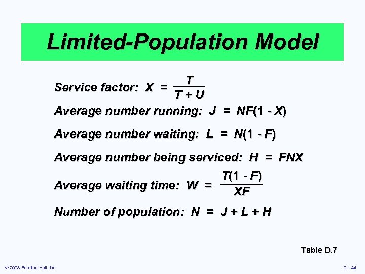 Limited-Population Model T T+U Average number running: J = NF(1 - X) Service factor: X = Average number waiting: L = N(1 - F) Average number being serviced: H = FNX T(1 - F) Average waiting time: W = XF Number of population: N = J + L + H Table D. 7 © 2008 Prentice Hall, Inc. D – 44
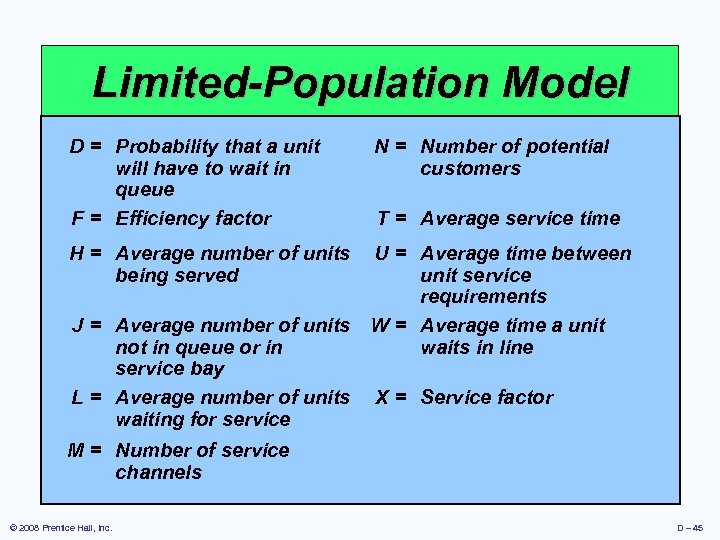 Limited-Population Model D = Probability that a unit N = Number of potential T will have to wait customers Service factor: in. X = T+U queue F = Average number running: J = NF(1 - X) time Efficiency factor T = Average service H = Averagenumber of waiting: =LAverage time between Average number units U = N(1 - F) being served unit service Average number being serviced: H = FNX requirements T(1 - F) J = Average number of units W = Average time a unit Average waiting time: W = waits in line not in queue or in XF service bay Number of population: N = J + L + H L = Average number of units X = Service factor waiting for service M = Number of service channels © 2008 Prentice Hall, Inc. D – 45
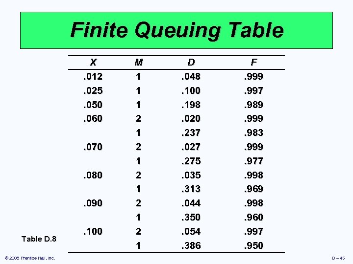 Finite Queuing Table X. 012. 025. 050. 060. 070. 080. 090 Table D. 8 © 2008 Prentice Hall, Inc. . 100 M 1 1 1 2 1 2 1 2 1 D. 048. 100. 198. 020. 237. 027. 275. 035. 313. 044. 350. 054. 386 F. 999. 997. 989. 999. 983. 999. 977. 998. 969. 998. 960. 997. 950 D – 46
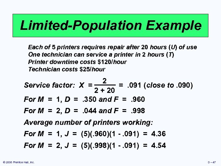 Limited-Population Example Each of 5 printers requires repair after 20 hours (U) of use One technician can service a printer in 2 hours (T) Printer downtime costs $120/hour Technician costs $25/hour 2 Service factor: X = =. 091 (close to. 090) 2 + 20 For M = 1, D =. 350 and F =. 960 For M = 2, D =. 044 and F =. 998 Average number of printers working: For M = 1, J = (5)(. 960)(1 -. 091) = 4. 36 For M = 2, J = (5)(. 998)(1 -. 091) = 4. 54 © 2008 Prentice Hall, Inc. D – 47
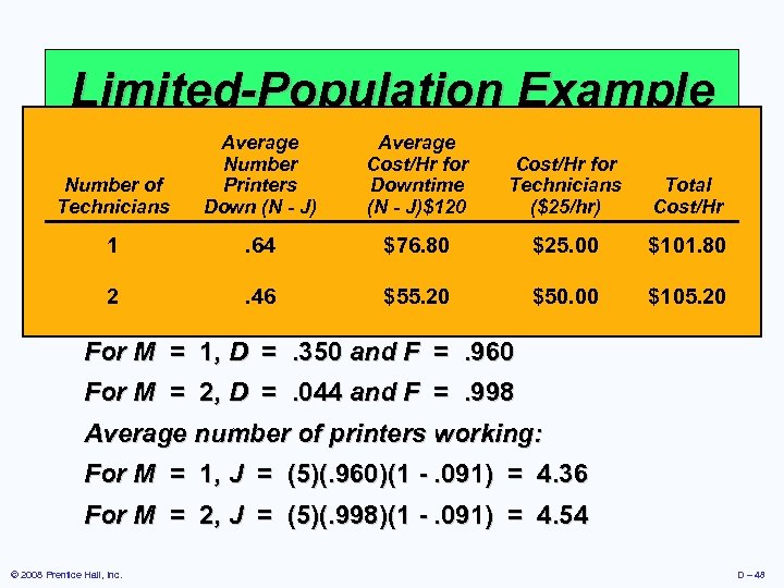 Limited-Population Example Average Number Each of 5 printers require Cost/Hrafter 20 Cost/Hr(for of use repair for hours U) Number of Printers Downtime Total Technicians One technician can service a printer in 2 hours (T) Technicians Down (N - J)$120 ($25/hr) Cost/Hr Printer downtime costs $120/hour Technician costs $25/hour $76. 80 1. 64 $25. 00 $101. 80 2 $55. 20 $50. 00 $105. 20 = =. 091 (close to. 090) 2 + 20 For M = 1, D =. 350 and F =. 960 2. 46 Service factor: X For M = 2, D =. 044 and F =. 998 Average number of printers working: For M = 1, J = (5)(. 960)(1 -. 091) = 4. 36 For M = 2, J = (5)(. 998)(1 -. 091) = 4. 54 © 2008 Prentice Hall, Inc. D – 48
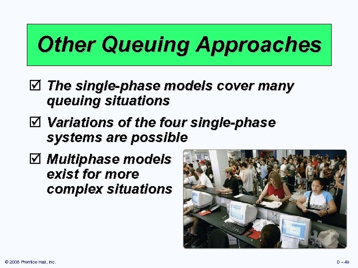 Other Queuing Approaches þ The single-phase models cover many queuing situations þ Variations of the four single-phase systems are possible þ Multiphase models exist for more complex situations © 2008 Prentice Hall, Inc. D – 49


