b8f2c559a2af496acfe1a5c169ce57a8.ppt
- Количество слайдов: 42
Operations Management Linear Programming Module B - Part 2 1
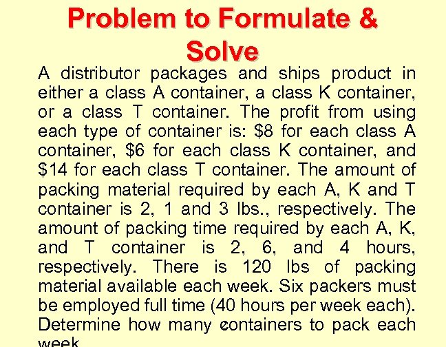
Problem to Formulate & Solve A distributor packages and ships product in either a class A container, a class K container, or a class T container. The profit from using each type of container is: $8 for each class A container, $6 for each class K container, and $14 for each class T container. The amount of packing material required by each A, K and T container is 2, 1 and 3 lbs. , respectively. The amount of packing time required by each A, K, and T container is 2, 6, and 4 hours, respectively. There is 120 lbs of packing material available each week. Six packers must be employed full time (40 hours per week each). 2 Determine how many containers to pack each
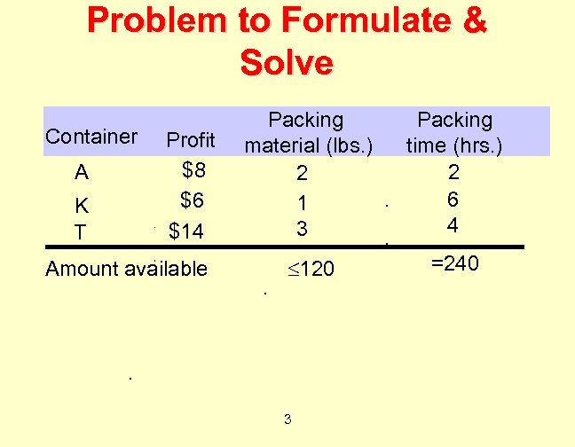
Problem to Formulate & Solve Container A K T Profit $8 $6 $14 Amount available Packing material (lbs. ) 2 1 3 Packing time (hrs. ) 2 6 4 120 =240 3
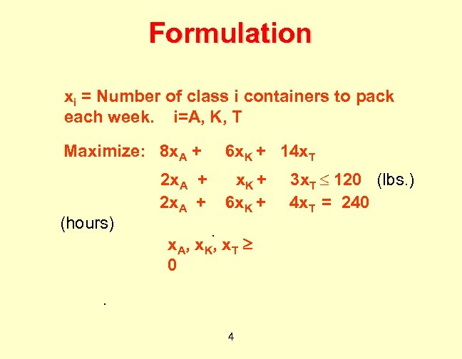
Formulation xi = Number of class i containers to pack each week. i=A, K, T Maximize: 8 x. A + (hours) 2 x. A + 6 x. K + 14 x. T x. K + 6 x. K + x A, x K, x T 0 4 3 x. T 120 (lbs. ) 4 x. T = 240
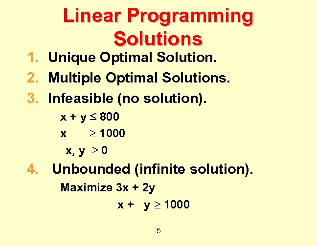
Linear Programming Solutions 1. Unique Optimal Solution. 2. Multiple Optimal Solutions. 3. Infeasible (no solution). x + y 800 x 1000 x, y 0 4. Unbounded (infinite solution). Maximize 3 x + 2 y x + y 1000 5
Computer Solutions ¨ Optimal values of decision variables and objective function. ¨ Sensitivity information for objective function coefficients. ¨ Sensitivity information for RHS (right -hand side) of constraints and shadow price. 6
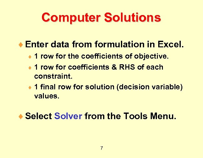
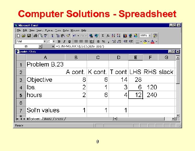
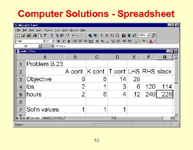
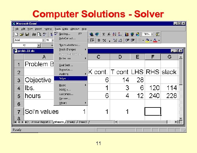
Computer Solutions ¨ Enter data from formulation in Excel. ¨ 1 row for the coefficients of objective. ¨ 1 row for coefficients & RHS of each constraint. ¨ 1 final row for solution (decision variable) values. ¨ Select Solver from the Tools Menu. 7
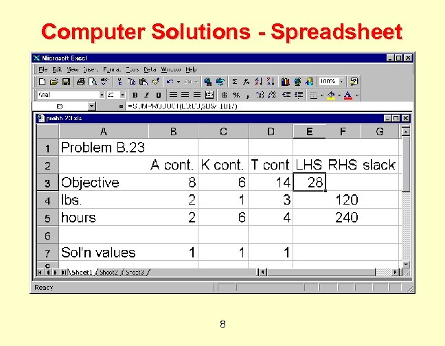
Computer Solutions - Spreadsheet 8
Computer Solutions - Spreadsheet 9
Computer Solutions - Spreadsheet 10
Computer Solutions - Solver 11
Computer Solutions - Solver 12
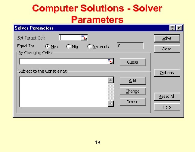
Computer Solutions - Solver Parameters 13
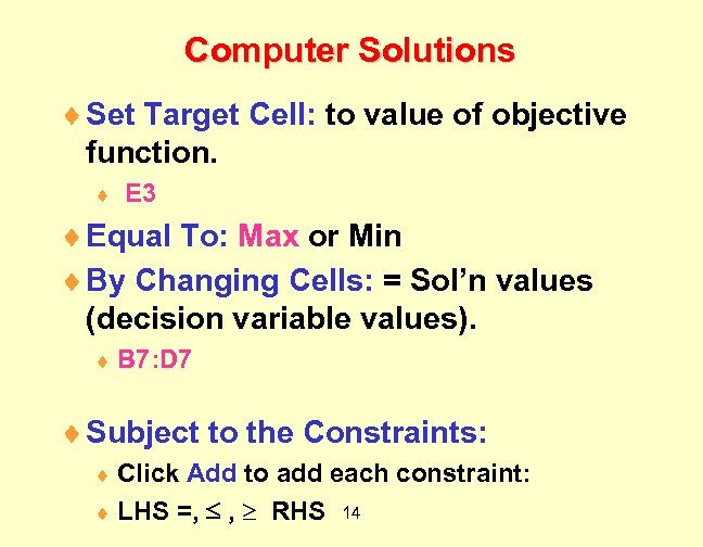
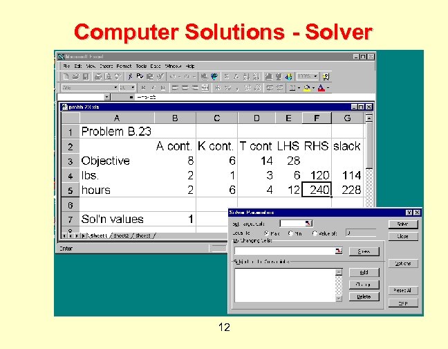
Computer Solutions ¨ Set Target Cell: to value of objective function. ¨ E 3 ¨ Equal To: Max or Min ¨ By Changing Cells: = Sol’n values (decision variable values). ¨ B 7: D 7 ¨ Subject to the Constraints: ¨ Click Add to add each constraint: ¨ LHS =, , RHS 14
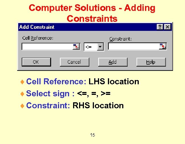
Computer Solutions - Adding Constraints ¨ Cell Reference: LHS location ¨ Select sign : <=, =, >= ¨ Constraint: RHS location 15
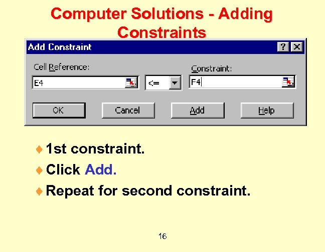
Computer Solutions - Adding Constraints ¨ 1 st constraint. ¨ Click Add. ¨ Repeat for second constraint. 16
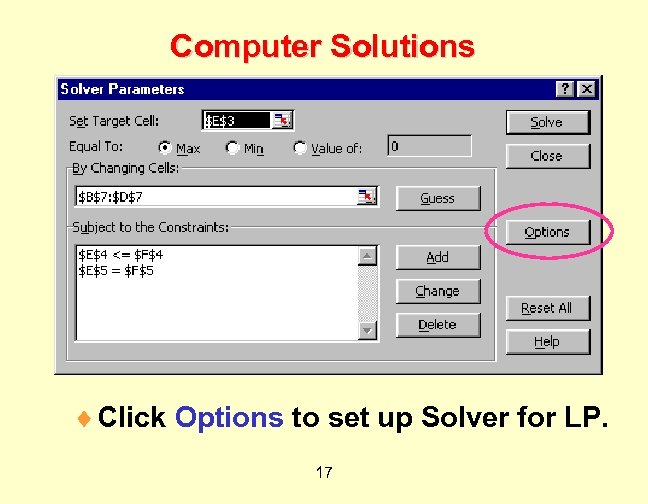
Computer Solutions ¨ Click Options to set up Solver for LP. 17
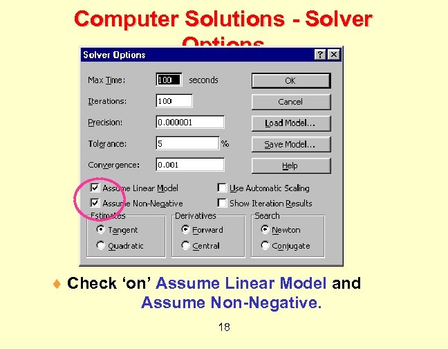
Computer Solutions - Solver Options ¨ Check ‘on’ Assume Linear Model and Assume Non-Negative. 18
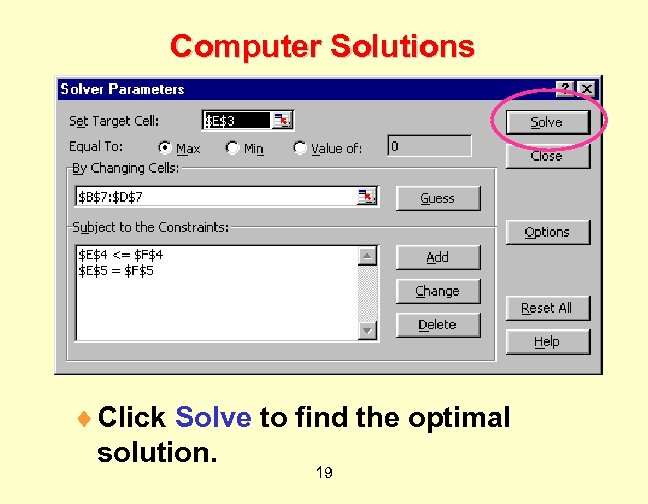
Computer Solutions ¨ Click Solve to find the optimal solution. 19
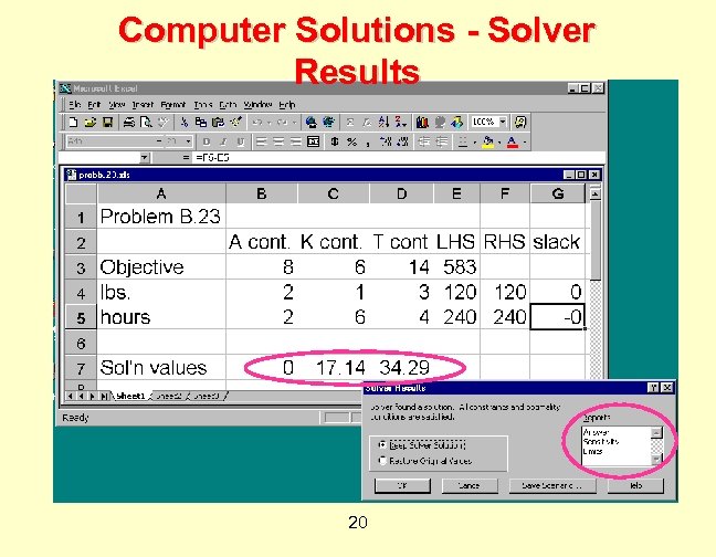
Computer Solutions - Solver Results 20
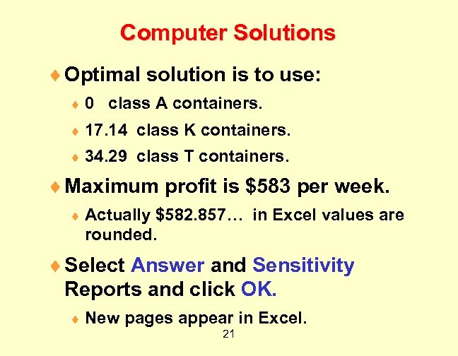
Computer Solutions ¨ Optimal solution is to use: ¨ 0 class A containers. ¨ 17. 14 class K containers. ¨ 34. 29 class T containers. ¨ Maximum profit is $583 per week. ¨ Actually $582. 857… in Excel values are rounded. ¨ Select Answer and Sensitivity Reports and click OK. ¨ New pages appear in Excel. 21
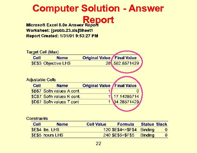
Computer Solution - Answer Report 22
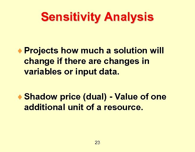
Sensitivity Analysis ¨ Projects how much a solution will change if there are changes in variables or input data. ¨ Shadow price (dual) - Value of one additional unit of a resource. 23
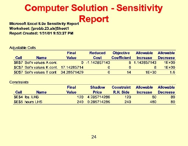
Computer Solution - Sensitivity Report 24
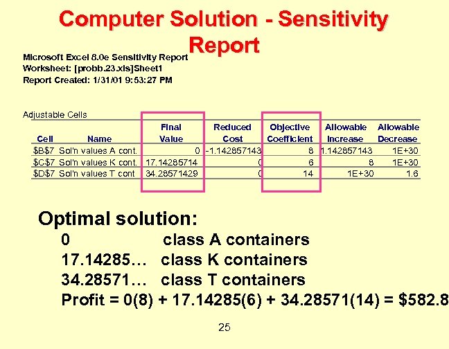
Computer Solution - Sensitivity Report Microsoft Excel 8. 0 e Sensitivity Report Worksheet: [probb. 23. xls]Sheet 1 Report Created: 1/31/01 9: 53: 27 PM Adjustable Cells Cell $B$7 $C$7 $D$7 Final Value Reduced Objective Allowable Name Cost Coefficient Increase Decrease Sol'n values A cont. 0 -1. 142857143 8 1. 142857143 1 E+30 Sol'n values K cont. 17. 14285714 0 6 8 1 E+30 Sol'n values T cont 34. 28571429 0 14 1 E+30 1. 6 Optimal solution: 0 class A containers 17. 14285… class K containers 34. 28571… class T containers Profit = 0(8) + 17. 14285(6) + 34. 28571(14) = $582. 8 25
Computer Solution - Sensitivity Report 26
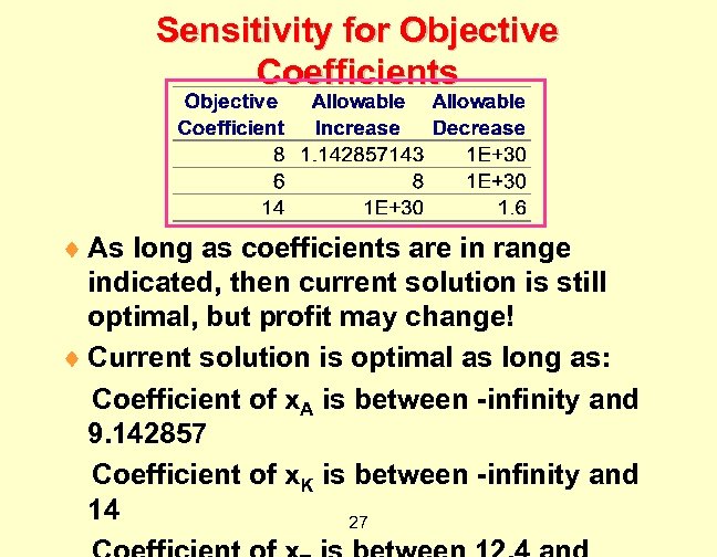
Sensitivity for Objective Coefficients ¨ As long as coefficients are in range indicated, then current solution is still optimal, but profit may change! ¨ Current solution is optimal as long as: Coefficient of x. A is between -infinity and 9. 142857 Coefficient of x. K is between -infinity and 14 27
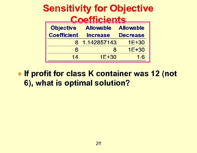
Sensitivity for Objective Coefficients ¨ If profit for class K container was 12 (not 6), what is optimal solution? 28
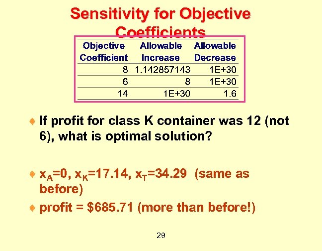
Sensitivity for Objective Coefficients ¨ If profit for class K container was 12 (not 6), what is optimal solution? ¨ x. A=0, x. K=17. 14, x. T=34. 29 (same as before) ¨ profit = $685. 71 (more than before!) 29

Sensitivity for Objective Coefficients ¨ If profit for class K container was 16 (not 6), what is optimal solution? 30
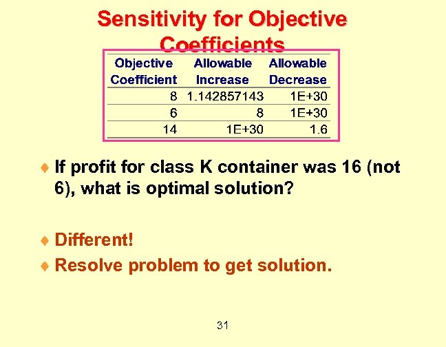
Sensitivity for Objective Coefficients ¨ If profit for class K container was 16 (not 6), what is optimal solution? ¨ Different! ¨ Resolve problem to get solution. 31
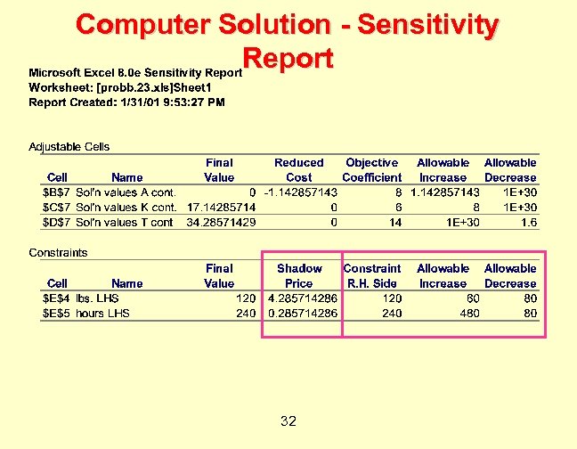
Computer Solution - Sensitivity Report 32
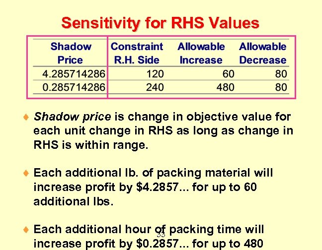
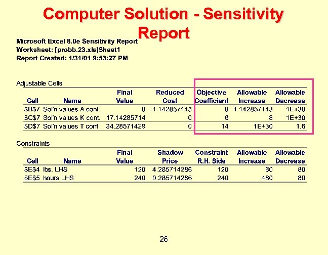
Sensitivity for RHS Values ¨ Shadow price is change in objective value for each unit change in RHS as long as change in RHS is within range. ¨ Each additional lb. of packing material will increase profit by $4. 2857. . . for up to 60 additional lbs. ¨ Each additional hour of packing time will 33 increase profit by $0. 2857. . . for up to 480
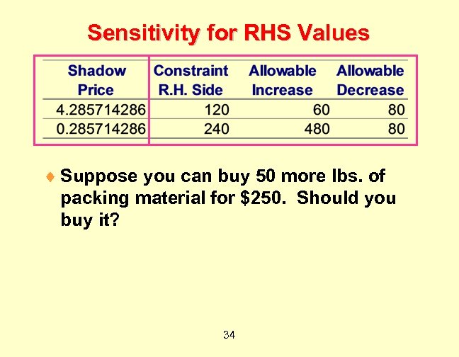
Sensitivity for RHS Values ¨ Suppose you can buy 50 more lbs. of packing material for $250. Should you buy it? 34
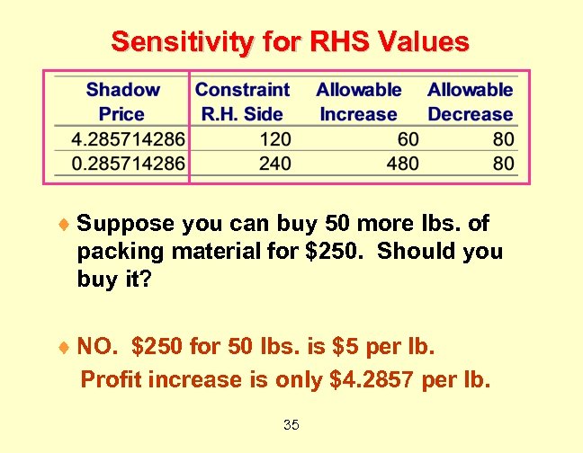
Sensitivity for RHS Values ¨ Suppose you can buy 50 more lbs. of packing material for $250. Should you buy it? ¨ NO. $250 for 50 lbs. is $5 per lb. Profit increase is only $4. 2857 per lb. 35
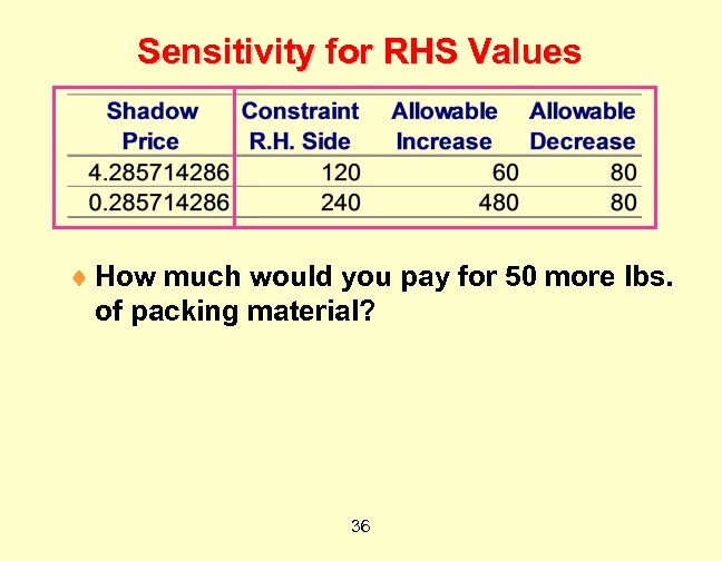
Sensitivity for RHS Values ¨ How much would you pay for 50 more lbs. of packing material? 36
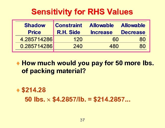
Sensitivity for RHS Values ¨ How much would you pay for 50 more lbs. of packing material? ¨ $214. 28 50 lbs. $4. 2857/lb. = $214. 2857. . . 37
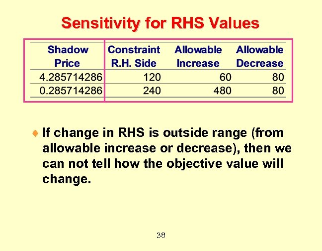
Sensitivity for RHS Values ¨ If change in RHS is outside range (from allowable increase or decrease), then we can not tell how the objective value will change. 38
Extensions of Linear Programming ¨ Integer programming (IP): Some or all variables are restricted to integer values. ¨ Allows ¨ Much “if…then” constraints. harder to solve (more computer time). ¨ Nonlinear programming: Some constraints or objective are nonlinear functions. ¨ Allows wider range of situations to be modeled. ¨ Much harder to solve (more computer time). 39
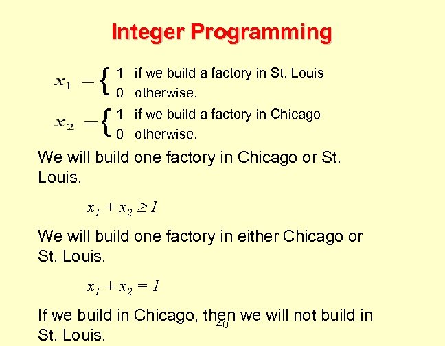
Integer Programming { 1 {0 1 if we build a factory in St. Louis 0 otherwise. if we build a factory in Chicago otherwise. We will build one factory in Chicago or St. Louis. x 1 + x 2 1 We will build one factory in either Chicago or St. Louis. x 1 + x 2 = 1 If we build in Chicago, then we will not build in 40 St. Louis.
New Formulation #1 You are creating an investment portfolio from 4 investment options: stocks, real estate, Tbills (Treasury-bills), and cash. Stocks have an annual rate of return of 12% and a risk measure of 5. Real estate has an annual rate of return of 10% and a risk measure of 8. Tbills have an annual rate of return of 5% and a risk measure of 1. Cash has an annual rate of return of 0% and a risk measure of 0. The average risk of the portfolio can not exceed 5. At least 15% of the portfolio must be in cash. Formulate an LP to maximize the annual rate 41 of return of the portfolio.
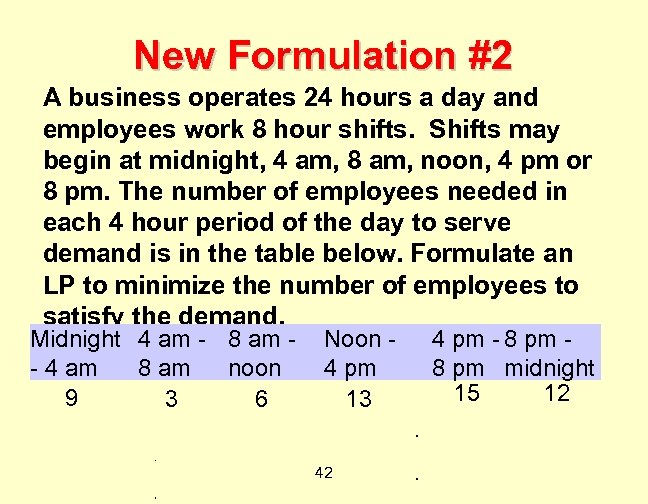
New Formulation #2 A business operates 24 hours a day and employees work 8 hour shifts. Shifts may begin at midnight, 4 am, 8 am, noon, 4 pm or 8 pm. The number of employees needed in each 4 hour period of the day to serve demand is in the table below. Formulate an LP to minimize the number of employees to satisfy the demand. Midnight 4 am - 8 am - 4 am 8 am noon 9 3 6 Noon 4 pm 13 42 4 pm - 8 pm midnight 15 12
b8f2c559a2af496acfe1a5c169ce57a8.ppt