e7b4478fcba209246230d1d845d17ff7.ppt
- Количество слайдов: 53
 On the Long-run Evolution of Inheritance France 1820 -2050 Thomas Piketty Paris School of Economics September 2010
 • There are two ways to become rich: either through one’s own work, or through inheritance • In the 19 th century and early 20 th, it was obvious to everybody that the 2 nd channel was important: inheritance and successors are everywhere in the literature; huge inheritance flow in tax data
 • Q: Does this belong to the past? Did modern growth kill the inheritance channel? E. g. rise of human capital and meritocracy? • This paper answers « NO » to this question and attempts to explains why, taking France 1820 -2050 as an illustration
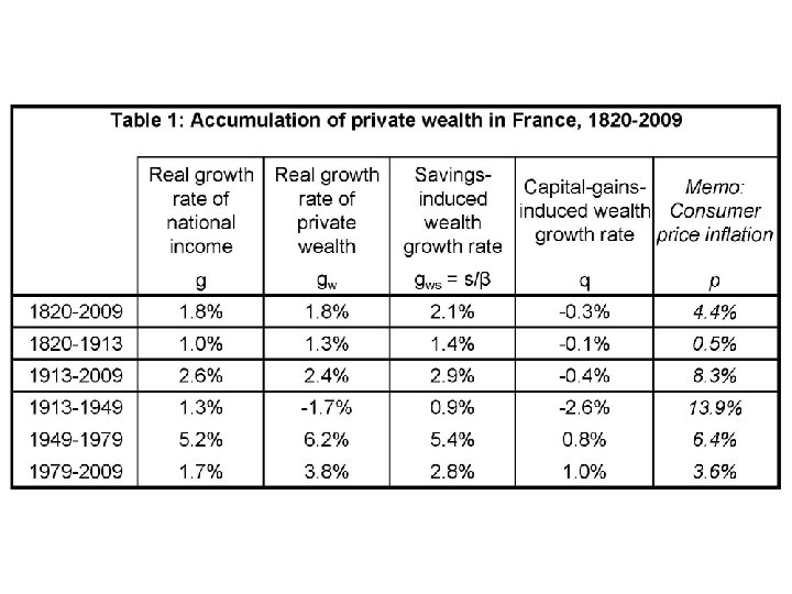
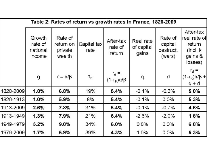
 What this paper does • Documents & explains this fact; draws lessons for other countries • Main lesson: with r>g (say, r=4%-5% vs g=1% -2%), then wealth coming from the past is being capitalized faster than growth, & inherited wealth dominates self-made wealth • Dynastic model: heirs save a fraction g/r of the return to inherited wealth, so that wealth-income ratio β=W/Y is stationary. Then steady-state bequest flow by=B/Y=β/H, with H= generation length. If β=600%, H=30 → by=20% • This can be generalized to more general saving models: if g small & r>g, then by close to β/H
 Application to the structure of lifetime inequality • Top incomes literature: Atkinson-Piketty OUP 2007 & 2010 → 23 countries. . but pb with capital side: we were not able to decompose labor-based vs inheritance-based inequality, i. e. meritocratic vs rentier societies → This paper = positive aggregate analysis; but building block for future work with heterogenity, inequality & optimal taxation
 Data sources • Estate tax data: aggregate data 18261964; tabulations by estate & age brackets 1902 -1964; national micro-files 1977 -1984 -1987 -1994 -2000 -2006; Paris micro-files 1807 -1932 • National wealth and income accounts: Insee official series 1949 -2009; linked up with various series 1820 -1949
 • French estate tax data is exceptionally good: universal, fully integrated bequest and gift tax since 1791 • Key feature: everybody has to fill a return, even with very low estates • 350, 000 estate tax returns/year in 1900 s and 2000 s, i. e. 65% of the 500, 000 decedents (US: < 2%) (memo: bottom 50% wealth share < 10%)
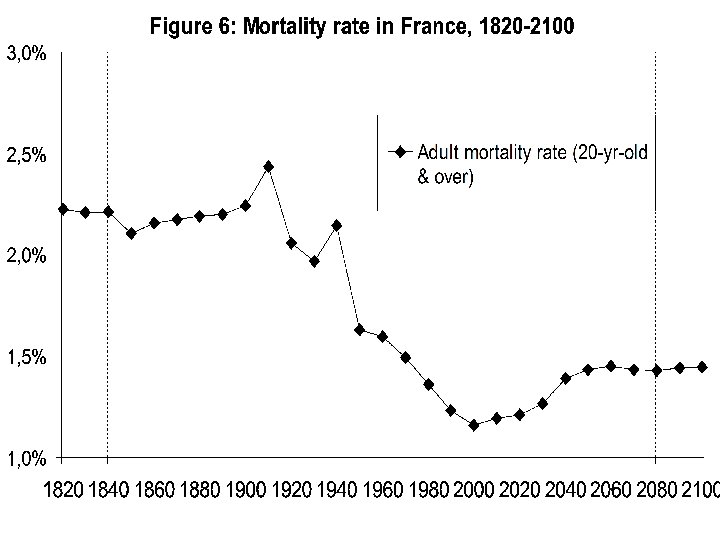
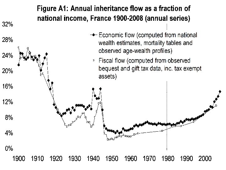
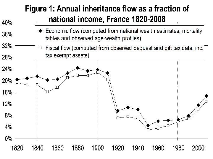
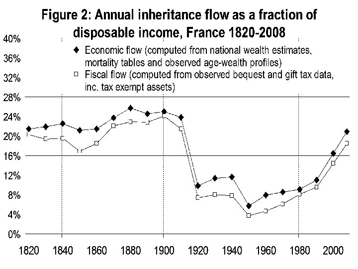
 Computing inheritance flow Bt/Yt = µt mt Wt/Yt ▪ Wt/Yt = aggregate wealth/income ratio ▪ mt = aggregate mortality rate ▪ µt = ratio between average wealth of decedents and average wealth of the living (= age-wealth profile) → The U-shaped pattern of inheritance is the product of three U-shaped effects
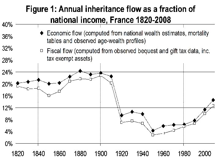
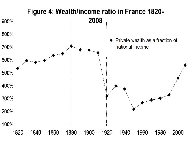
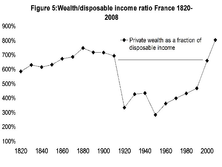
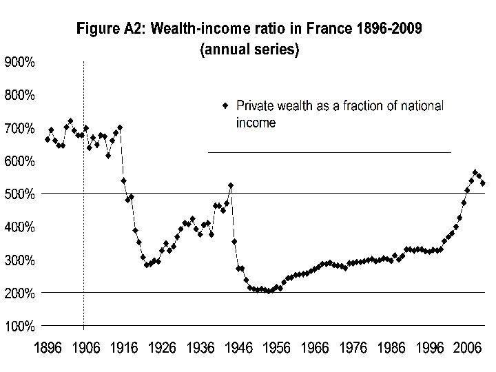
 • 1900 s: Y = 35 billions francs or, W = 250 billions, B = 8. 5 billions → W/Y = 700%, B/Y = 25% • 2008: Y = 1 700 billions € (i. e. 35 000€ per adult), W = 9 500 billions € (200 000€ per adult), B = 240 billions € → W/Y = 560%, B/Y = 15% • Between 1900 s and 1950 s, W/Y divided by 3, but B/Y divided by 6 → the fall in W/Y explains about half of the fall in B/Y
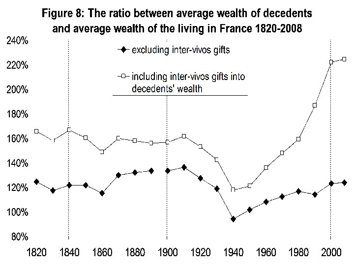
 Table 2: Raw age-wealth-at-death profiles in France, 18202008 20 -29 30 -39 40 -49 50 -59 60 -69 70 -79 80+ 1827 50% 63% 73% 100% 113% 114% 122% 1857 57% 58% 86% 100% 141% 125% 154% 1887 45% 33% 63% 100% 152% 213% 225% 1902 26% 57% 78% 100% 172% 176% 233% 1912 23% 54% 74% 100% 158% 176% 237% 1931 22% 59% 77% 100% 123% 137% 143% 1947 23% 52% 77% 100% 99% 76% 62% 1960 28% 52% 74% 100% 110% 101% 87% 1984 19% 55% 83% 100% 118% 113% 105% 2000 19% 46% 66% 100% 122% 121% 118%
 How can we account for these facts? • 1914 -45 capital shocks played a big role, and it took a long time to recover • Key question: why does the age-wealth profile become upward-sloping again? → the r>g effect • Where does the B/Y=20%-25% magic number come from? Why µt ↑ seem to compensate exactly mt ↓?
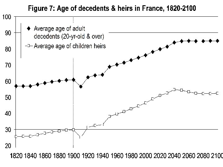
 Theory 1: Demography • To simplify: deterministic, stationary demographic structure: everybody becomes adult at age A, has one kid at age H, inherits at age I, and dies at age D • 1900: A=20, H=30, D=60 → I=D-H=30 • 2050: A=20, H=30, D=80 → I=D-H=50 • mortality rate among adults: mt = 1/(D-A) (1900: about 2. 5%; 2050: about 1. 7%)
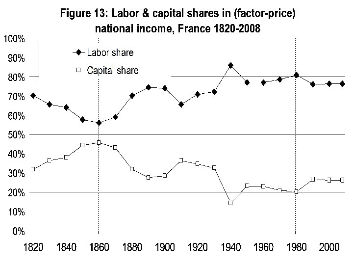
 = F(Kt , egt Lt)") Theory 2: Production • Yt = F(Kt , Ht) = F(Kt , egt Lt) • g = exogenous productivity growth rate • E. g. Cobb-Douglas: F(K, H) = Kα H 1 -α • Yt = YKt + YLt , with YKt = rt Kt = αt Yt • Define βt = Kt/Yt = Wt/Yt (closed economy) (open economy: Wt = Kt + FWt) (+Dt) • Then αt = rt βt , i. e. rt = αt/βt • E. g. if βt = 600%, αt =30%, then rt = 5%
Theory 2: Production • Yt = F(Kt , Ht) = F(Kt , egt Lt) • g = exogenous productivity growth rate • E. g. Cobb-Douglas: F(K, H) = Kα H 1 -α • Yt = YKt + YLt , with YKt = rt Kt = αt Yt • Define βt = Kt/Yt = Wt/Yt (closed economy) (open economy: Wt = Kt + FWt) (+Dt) • Then αt = rt βt , i. e. rt = αt/βt • E. g. if βt = 600%, αt =30%, then rt = 5%
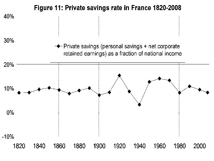
 Theory 3: Savings • Aggregate savings rate = stable at about 10% of Yt since 1820 → β* = s/g (g=1% & s=6% → β* = 600%) • Exogenous saving: St = s. Yt = s. LYLt + s. Kr. Wt • Is s. K>s. L? • Dynastic utility function: s. K=g/r, s. L=0 • Bequest in the utility function: U(C, B) → easy to generate s. K > s. L (or s. K
 → Ramsey") • Dynastic model: U = ∫ e-θt Ct 1 -σ/(1 -σ) → Ramsey steady-state: r* = θ + σg (> g) • In effect: s. L*=0%, s. K=g/r*% • Any wealth distribution s. t. f’(k*)=r* is a steady-state • Intuition: YLt grows at rate g, workers don’t need to save; but capitalists need to save a fraction g/r of their capital income YKt= r Wt , so that Wt grows at rate g
• Dynastic model: U = ∫ e-θt Ct 1 -σ/(1 -σ) → Ramsey steady-state: r* = θ + σg (> g) • In effect: s. L*=0%, s. K=g/r*% • Any wealth distribution s. t. f’(k*)=r* is a steady-state • Intuition: YLt grows at rate g, workers don’t need to save; but capitalists need to save a fraction g/r of their capital income YKt= r Wt , so that Wt grows at rate g
 at") Steady-state age-wealth profile • If s. L=0%, then the cross-sectional agewealth profile Wt(a) at time t is very simple: - If A
Steady-state age-wealth profile • If s. L=0%, then the cross-sectional agewealth profile Wt(a) at time t is very simple: - If A
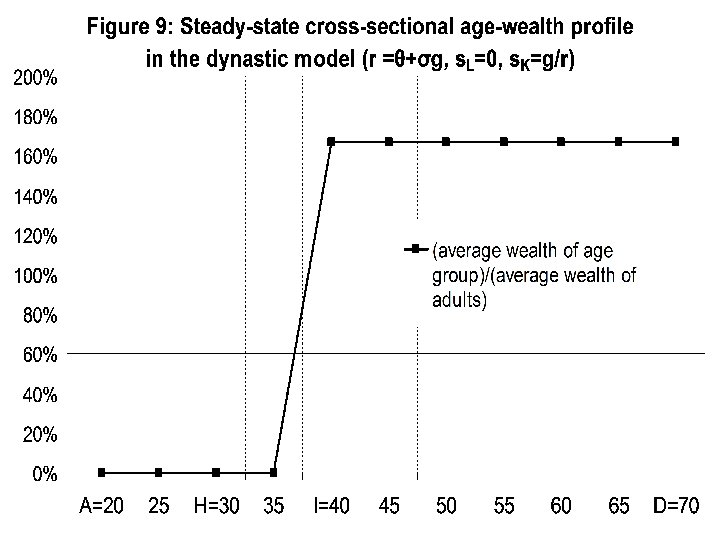
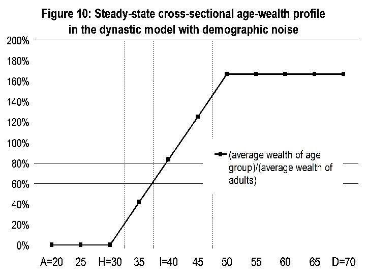
, s. L=0, s. K=g/r, µ=(D-A)/H") Proposition 1: Steady-state of dynastic model : r=θ+σg (>g), s. L=0, s. K=g/r, µ=(D-A)/H (>1) → B/Y is independant of life expectancy: µ = (D-A)/H, m=1/(D-A), so B/Y = µ m W/Y = β/H E. g. if β=600%, H=30, then B/Y=20% 1900: D=60, I=30, m=2. 5%, but µ=133% 2050: D=80, I=50, m=1. 6%, but µ=200%» Proposition 2: More generally: µ = [1 -e-(g-s r)(D-A)]/[1 -e-(g-s r)(D-I)] → µ’(s. K)>0, µ’(r)>0, µ’(g)<0 (→ for g small, µ close to (D-A)/H) K K
Proposition 1: Steady-state of dynastic model : r=θ+σg (>g), s. L=0, s. K=g/r, µ=(D-A)/H (>1) → B/Y is independant of life expectancy: µ = (D-A)/H, m=1/(D-A), so B/Y = µ m W/Y = β/H E. g. if β=600%, H=30, then B/Y=20% 1900: D=60, I=30, m=2. 5%, but µ=133% 2050: D=80, I=50, m=1. 6%, but µ=200%» Proposition 2: More generally: µ = [1 -e-(g-s r)(D-A)]/[1 -e-(g-s r)(D-I)] → µ’(s. K)>0, µ’(r)>0, µ’(g)<0 (→ for g small, µ close to (D-A)/H) K K
 in 1820 or 1900") Simulations • I start from the observed age-wealth profile Wt(a) in 1820 or 1900 • I take st and rt from national accounts • I take observed age-labor income (+transfer income) profiles • I apply observed mortality rates by age group, and observed age structure of heirs, donors and donees • I try different savings behavior to replicate observed dynamics of µt & Bt/Yt
Simulations • I start from the observed age-wealth profile Wt(a) in 1820 or 1900 • I take st and rt from national accounts • I take observed age-labor income (+transfer income) profiles • I apply observed mortality rates by age group, and observed age structure of heirs, donors and donees • I try different savings behavior to replicate observed dynamics of µt & Bt/Yt
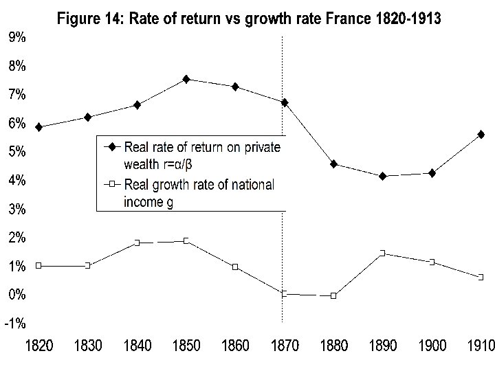
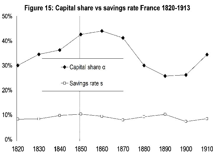
 Simulations 1: 19 th century • France 1820 -1910 = quasi-steady-state • β = W/Y = 629%, g=1. 0%, s=10. 1%, α=38% → r = 6. 0% >> g=1. 0% • Key fact about 19 th century growth = rate of return r much bigger than g → wealth holders only need to save a small fraction of their capital income to maintain a constant or rising W/Y ( gw=s/β=1. 3% → W/Y was slightly rising)
 → in order to reproduce both the 1820 -1910 pattern of B/Y and the observed agewealth profile (rising at high ages), one needs to assume that most of the savings came from capital income (i. e. s. L close to 0 and s. K close to g/r) (consistent with high wealth concentration of the time)
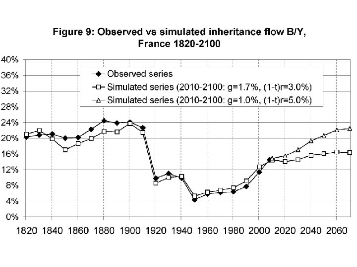
 Simulations 2: 20 th & 21 st centuries • Uniform savings s=s. K=s. L can reproduce both B/Y & observed age-wealth profiles over 1900 -2008 • 2010 -2050 simulations: g=1. 7%, s=9. 4%, α=26%, after-tax r=3. 0% → B/Y stabilizes at 16% • But if g=1. 0% & after-tax r=4. 5% (rising global k share and/or k tax cuts), then B/Y converges towards 22%-23%
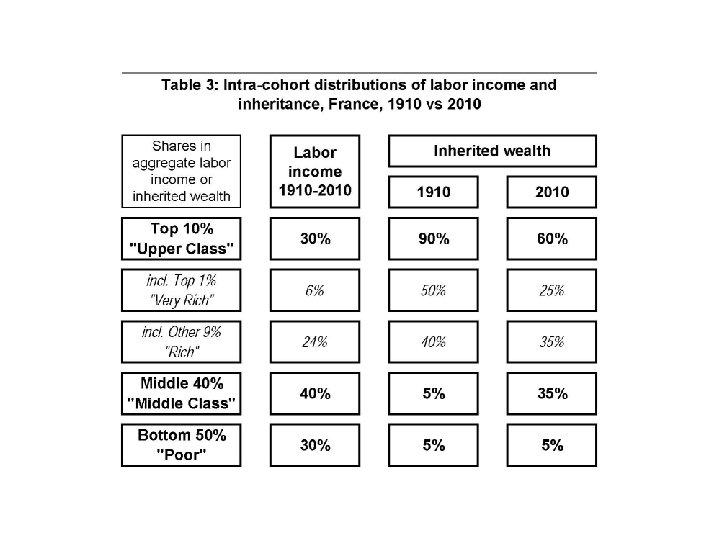
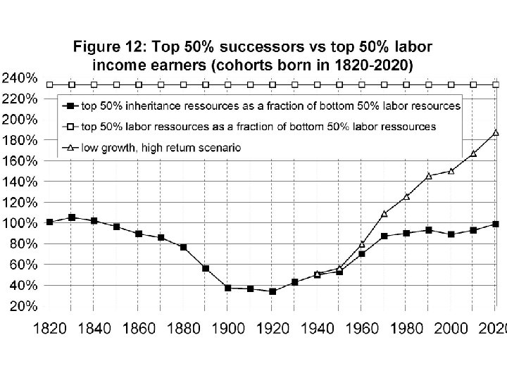
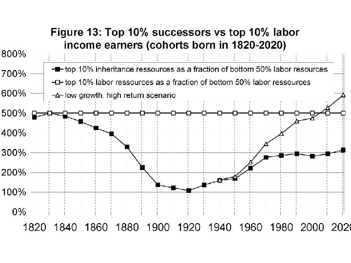
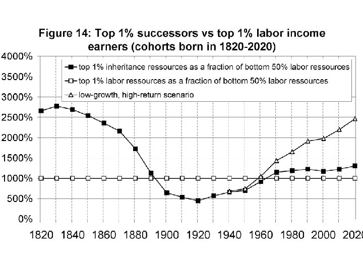
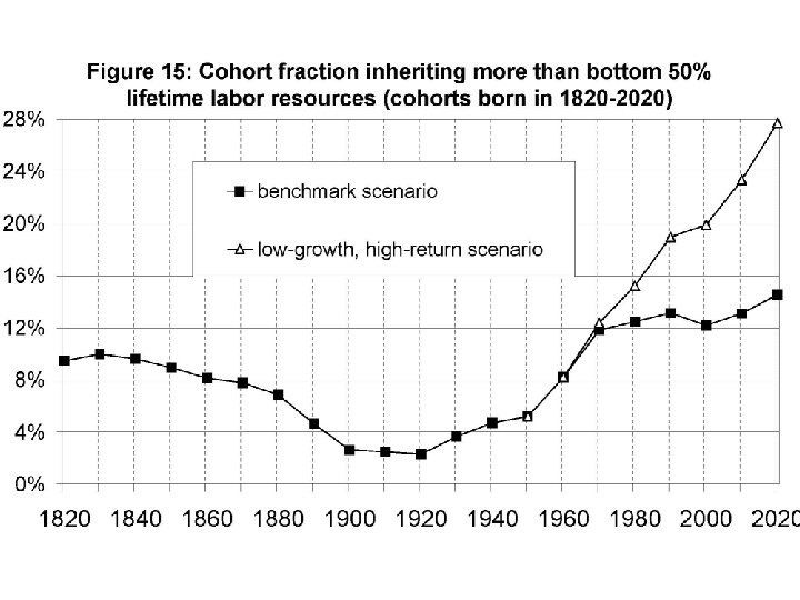
 Applications to distributional analysis • 19 c: top successors dominate top labor earners; top 1% spouse > top 1% job • Cohorts born in 1900 s-1950 s: for the first time maybe in history, top labor incomes dominate top successors • Cohorts born in 1970 s-1980 s & after: closer to 19 c rentier society than to 20 c meritocratic society. E. g. with labor income alone, hard to buy an appartment in Paris. .
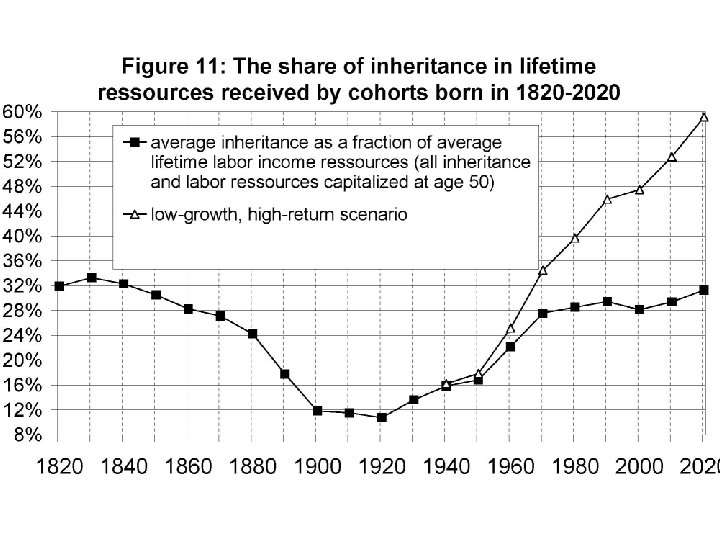
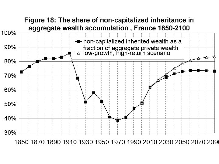
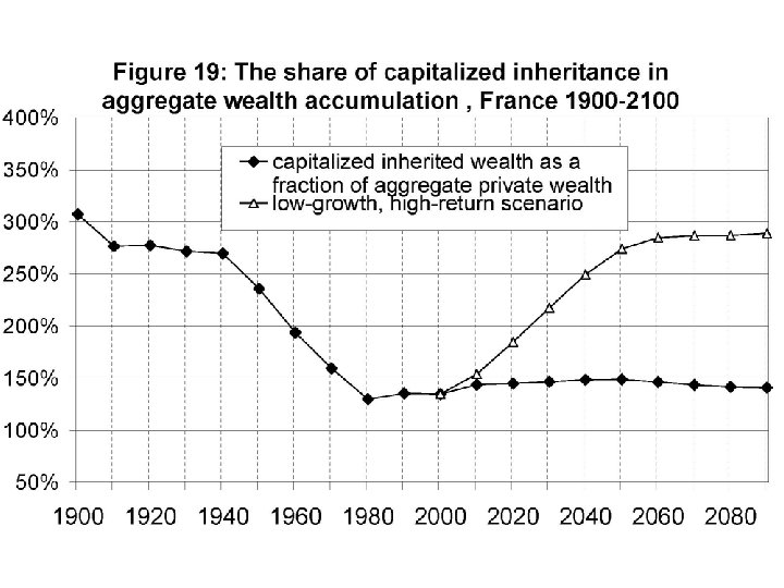
 Application to the share of inheritance in total wealth • Modigliani AER 1986, JEP 1988: inheritance = 20% of total U. S. wealth • Kotlikoff-Summers JPE 1981, JEP 1988: inheritance = 80% of total U. S. wealth • Three problems: - Bad data - We do not live in a stationary world: lifecycle wealth was much more important in the 1950 s-1970 s than it is today - We do not live in a representative-agent world → new definition of inheritance share
 What have we learned? • Capital accumulation takes time; one should not look at past 10 or 20 yrs and believe this is steady-state; life cycle theorists were too much influenced by what they saw in the 1950 s-1970 s… • Inheritance is likely to be a big issue in the 21 st century • Modern economic growth did not kill inheritance; the rise of human capital simply did not happen; g>0 but small not very different from g=0
 • A lot depends on r vs g+n: → China/India: inheritance doesn’t matter → US: inheritance smaller than in Europe → Italy, Spain, Germany (n<0): U-shaped pattern probably even bigger than France → world, very long run: g+n=0%: inheritance and past wealth will play a dominant role; back to 19 th century intuitions • But no normative model… difficult conceptual issues before we have good optimal k tax theory (endogenous r) → see Piketty-Saez, in progress…