Object Recognition CS 485 685 Computer Vision Dr George

Object Recognition CS 485/685 Computer Vision Dr. George Bebis

Object Recognition • Model-based Object Recognition • Generic Object Recognition

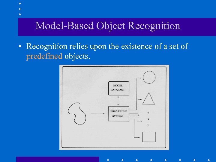
Model-Based Object Recognition • Recognition relies upon the existence of a set of predefined objects.

Generic Object Recognition (or Object Categorization)

Main Steps • Preprocessing – A model database is built by establishing associations between features and models. • Recognition – Scene features are used to retrieve appropriate associations stored in the model database.

Challenges • The appearance of an object can have a large range of variation due to: – – viewpoint changes shape changes (e. g. , non-rigid objects) photometric effects scene clutter • Different views of the same object can give rise to widely different images!

Requirements • Invariance – Geometric transformations (translation, rotation, scale) • Caused by viewpoint changes due to camera/object motion • Robustness – – – Noise (i. e. , sensor noise) Detection errors (e. g. , edge or corner detection) Illumination/Shadows Partial occlusion (i. e. , self and from other objects) Intrinsic shape distortions (i. e. , non-rigid objects)

Performance Criteria (1) Scope – What kind of objects can be recognized and in what kind of scenes ? (2) Robustness – Does the method tolerate reasonable amounts of noise and occlusion in the scene ? – Does it degrade gracefully as those tolerances are exceeded ?

Performance Criteria (cont’d) (3) Efficiency – How much time and memory are required to search the solution space ? (4) Accuracy – Correct recognition – False positives (wrong recognitions) – False negatives (missed recognitions)

Approaches Differ According To: • Restrictions on the form of the objects – 2 D or 3 D objects – Simple vs complex objects – Rigid vs deforming objects • Representation schemes – Object-centered – Viewer-centered

Approaches Differ According To: (cont’d) • Matching scheme – Geometry-based (i. e. , shape) – Appearance-based (e. g. , eigenfaces) • Type of features – Local (i. e. , SIFT) – Global (e. g. , eigen-coefficients)

Approaches Differ According To: (cont’d) • Image formation model – Perspective projection – Orthographic projection + scale – Affine transformation (e. g. , for planar objects)

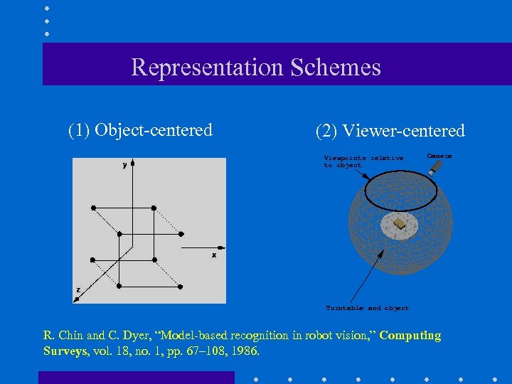
Representation Schemes (1) Object-centered (2) Viewer-centered R. Chin and C. Dyer, “Model-based recognition in robot vision, ” Computing Surveys, vol. 18, no. 1, pp. 67– 108, 1986.

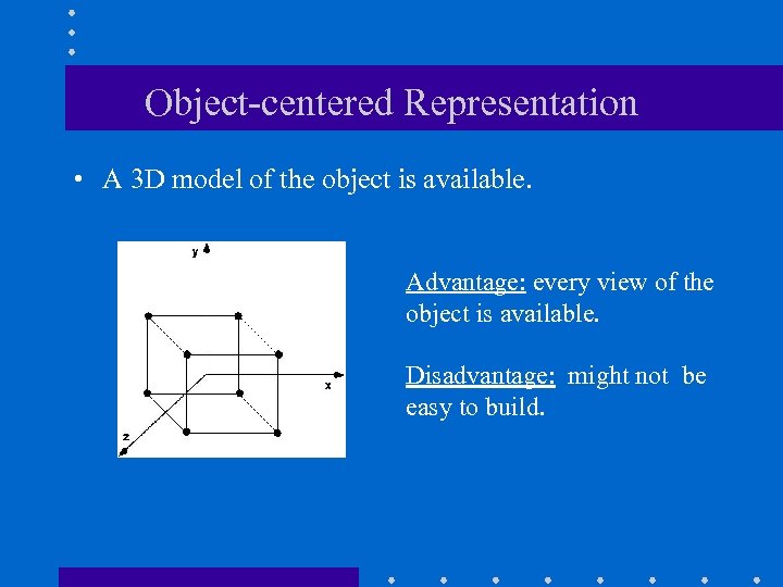
Object-centered Representation • A 3 D model of the object is available. Advantage: every view of the object is available. Disadvantage: might not be easy to build.

Object-centered Representation (cont’d) • Two different matching approaches: (1) (3 D/3 D): reconstruct object from the scene and match it with the models. e. g. , using “shape from X” methods (2) (3 D/2 D): back-project candidate model onto the scene and match it with the objects in the scene. i. e. , requires camera calibration

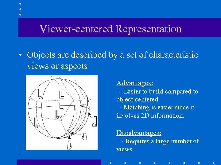
Viewer-centered Representation • Objects are described by a set of characteristic views or aspects Advantages: - Easier to build compared to object-centered. - Matching is easier since it involves 2 D information. Disadvantages: - Requires a large number of views.

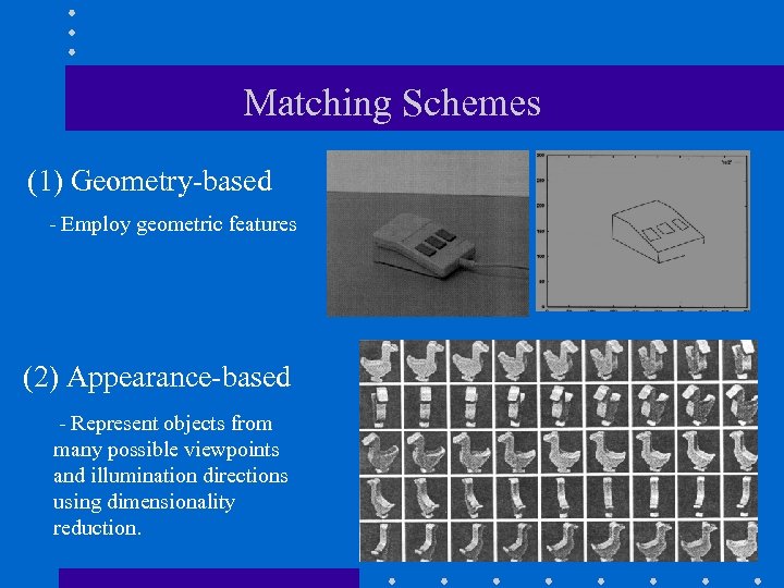
Matching Schemes (1) Geometry-based - Employ geometric features (2) Appearance-based - Represent objects from many possible viewpoints and illumination directions using dimensionality reduction.

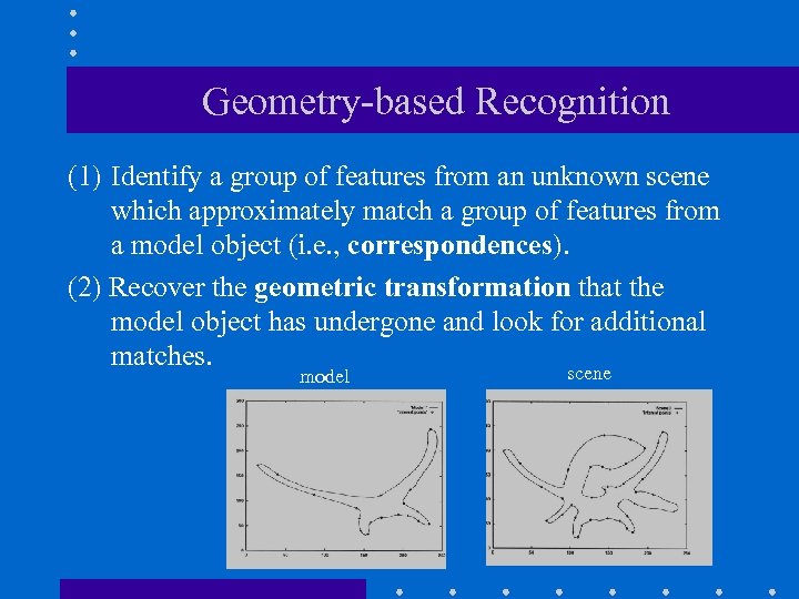
Geometry-based Recognition (1) Identify a group of features from an unknown scene which approximately match a group of features from a model object (i. e. , correspondences). (2) Recover the geometric transformation that the model object has undergone and look for additional matches. scene model

2 D Transformation Spaces • Rigid transformations (3 parameters) • Similarity transformations (4 parameters) • Affine transformations (6 parameters)

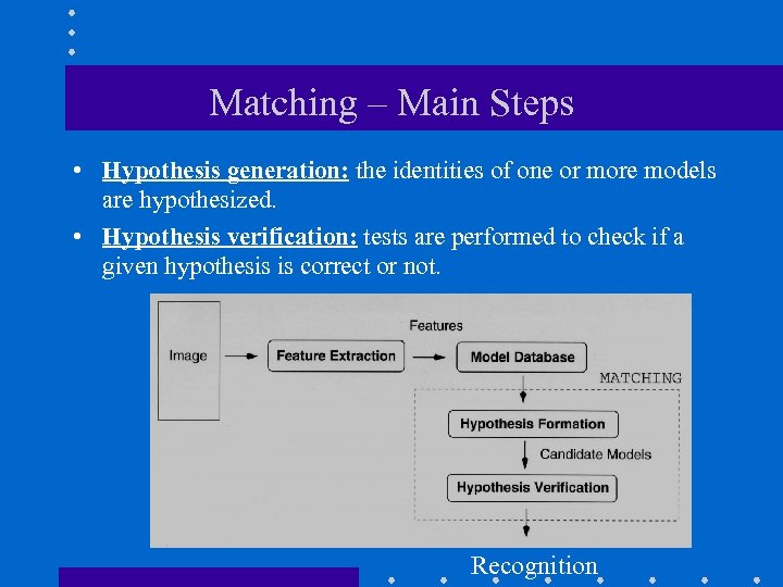
Matching – Main Steps • Hypothesis generation: the identities of one or more models are hypothesized. • Hypothesis verification: tests are performed to check if a given hypothesis is correct or not. Recognition

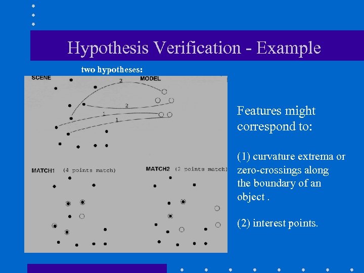
Hypothesis Verification - Example two hypotheses: Features might correspond to: (1) curvature extrema or zero-crossings along the boundary of an object. (2) interest points.

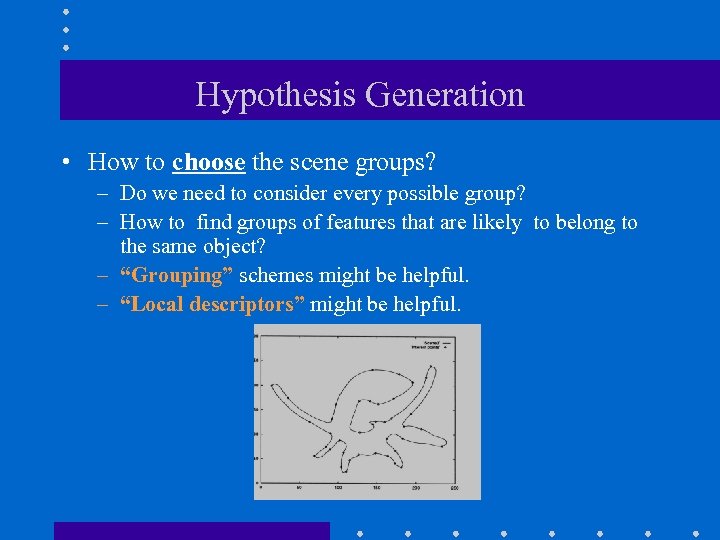
Hypothesis Generation • How to choose the scene groups? – Do we need to consider every possible group? – How to find groups of features that are likely to belong to the same object? – “Grouping” schemes might be helpful. – “Local descriptors” might be helpful.

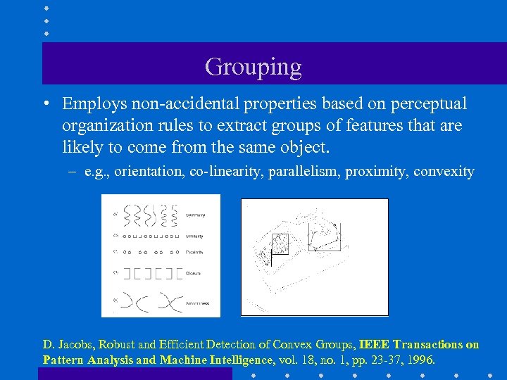
Grouping • Employs non-accidental properties based on perceptual organization rules to extract groups of features that are likely to come from the same object. – e. g. , orientation, co-linearity, parallelism, proximity, convexity D. Jacobs, Robust and Efficient Detection of Convex Groups, IEEE Transactions on Pattern Analysis and Machine Intelligence, vol. 18, no. 1, pp. 23 -37, 1996.

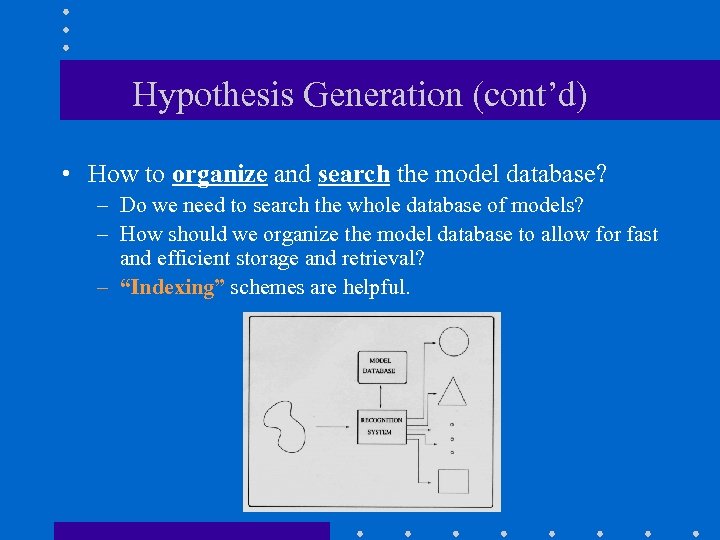
Hypothesis Generation (cont’d) • How to organize and search the model database? – Do we need to search the whole database of models? – How should we organize the model database to allow for fast and efficient storage and retrieval? – “Indexing” schemes are helpful.

We will discuss … • Alignment • Pose Clustering • Geometric Hashing (i. e. , indexing-based)

Recognition by Alignment • The alignment approach seeks to recover the geometric transformation between the model and the scene using a minimum number of correspondences. • Assuming affine transformations, three correspondences are enough. D. Huttenlocher and S. Ullman, "Object Recognition Using Alignment, International Conference on Computer Vision, pp. 102 -111, 1987.

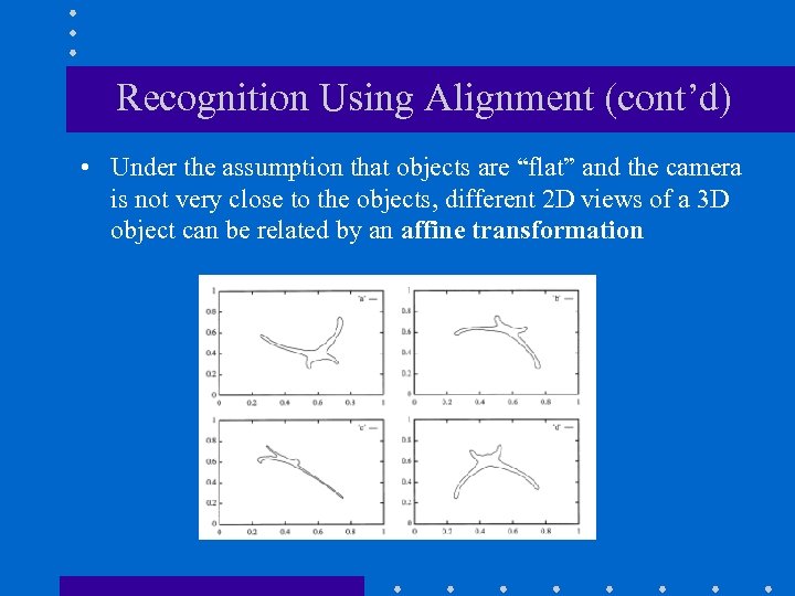
Recognition Using Alignment (cont’d) • Under the assumption that objects are “flat” and the camera is not very close to the objects, different 2 D views of a 3 D object can be related by an affine transformation

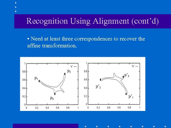
Recognition Using Alignment (cont’d) • Need at least three correspondences to recover the affine transformation. p 2 p’ 3 p 1 p’ 2 p 3 p’ 1

Recognition Using Pose Clustering • Performs “voting” in transformation space: - Correct transformations bring into alignment a large number of features. - Incorrect transformations bring into alignment a small number of features. • Transformations that can bring into alignment a large number of features, will receive a large number of votes (i. e. , support). C. Olson, "Efficient Pose Clustering Using a Randomized Algorithm“, International Journal of Computer Vision, vol. 23, no. 2, pp. 131 -147, 1997.

Pose Clustering (cont’d) • Main Steps (1) Quantize the space of possible transformations (usually 4 D - 6 D). (2) For each hypothetical match, solve for the transformation that aligns the matched features. (3) Cast a “vote” in the corresponding transformation space bin. (4) Find "peak" in transformation space.

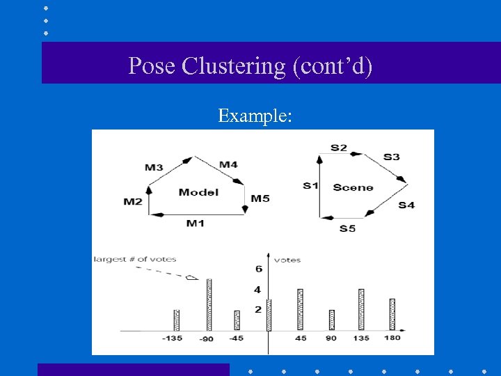
Pose Clustering (cont’d) Example:

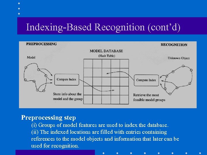
Indexing-Based Recognition (cont’d) Preprocessing step (i) Groups of model features are used to index the database. (ii) The indexed locations are filled with entries containing references to the model objects and information that later can be used for recognition.

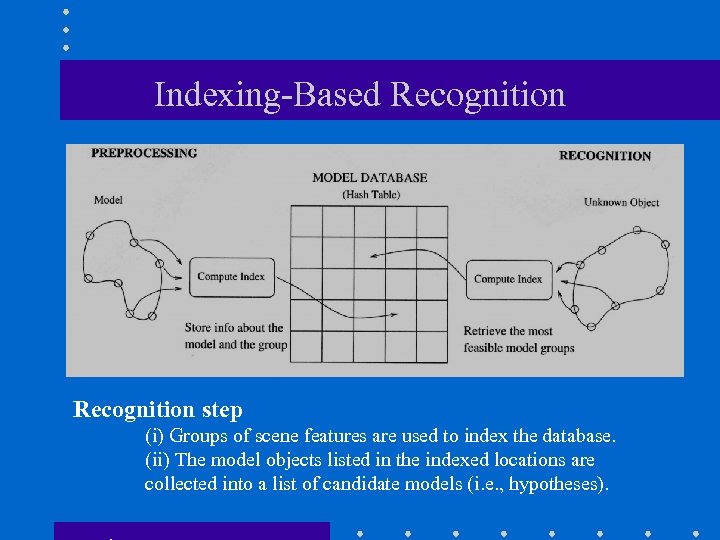
Indexing-Based Recognition step (i) Groups of scene features are used to index the database. (ii) The model objects listed in the indexed locations are collected into a list of candidate models (i. e. , hypotheses).

Indexing-Based Recognition (cont’d) • Ideally, we would like the index computed from a group of model features to be invariant. – i. e. , its properties will not change with object transformations or viewpoint changes. • Only one entry per group needs to be stored!

Geometric Hashing • Indexing using affine invariants. • Index remains invariant under affine transformations. Y. Lamdan, J. Schwartz, and H. Wolfson, "Affine invariant model-based object recognition" , IEEE Transactions on Robotics and Automation, vol. 6, no. 5, 1990. 2. H. Wolfson and I. Rigoutsos, "Geometric Hashing: An Overview" , IEEE Computational Science and Engineering, pp. 10 -21, October-December 1997.

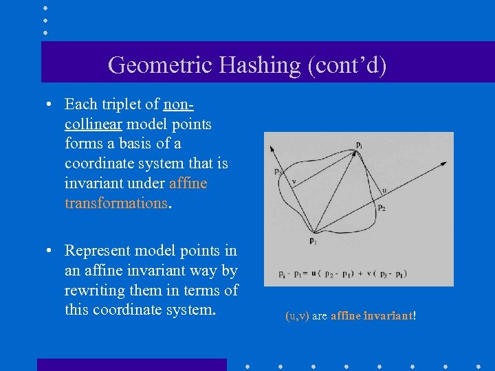
Geometric Hashing (cont’d) • Each triplet of noncollinear model points forms a basis of a coordinate system that is invariant under affine transformations. • Represent model points in an affine invariant way by rewriting them in terms of this coordinate system. (u, v) are affine invariant!

Geometric Hashing (cont’d) (model, (p 1, p 2, p 3))

Geometric Hashing: Preprocessing Step For each model do: (1) Extract a set of interest points. (2) For each ordered set of three, non-collinear, points (p 1, p 2, p 3) (2 a) Compute the coordinates (u, v) of the remaining features in the coordinate frame defined by the model basis (p 1, p 2, p 3) (2 b) After proper scaling and quantization, use the computed coordinates (u, v) as an index to a two dimensional hash table, and record in the corresponding hash table bin the information (model, (p 1, p 2, p 3))

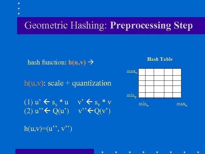
Geometric Hashing: Preprocessing Step Hash Table hash function: h(u, v) maxv h(u, v): scale + quantization (1) u’ su * u v’ sv * v (2) u’’ Q(u’) v’’ Q(v’) h(u, v)=(u’’, v’’) miny minu maxu

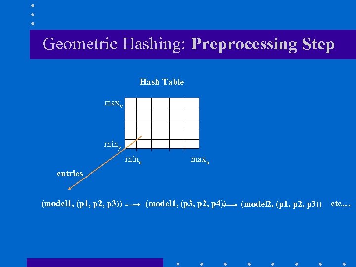
Geometric Hashing: Preprocessing Step Hash Table maxv miny minu maxu entries (model 1, (p 1, p 2, p 3)) (model 1, (p 3, p 2, p 4)) (model 2, (p 1, p 2, p 3)) etc…

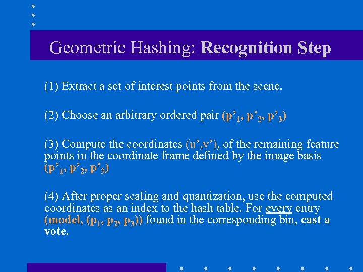
Geometric Hashing: Recognition Step (1) Extract a set of interest points from the scene. (2) Choose an arbitrary ordered pair (p’ 1, p’ 2, p’ 3) (3) Compute the coordinates (u’, v’), of the remaining feature points in the coordinate frame defined by the image basis (p’ 1, p’ 2, p’ 3) (4) After proper scaling and quantization, use the computed coordinates as an index to the hash table. For every entry (model, (p 1, p 2, p 3)) found in the corresponding bin, cast a vote.

Geometric Hashing (cont’d) (model, (p 1, p 2, p 3))

Geometric Hashing: Preprocessing Step Hash Table maxv miny minu maxu entries (model 1, (p 1, p 2, p 3)) (model 1, (p 3, p 2, p 4)) (model 2, (p 1, p 2, p 3)) etc…

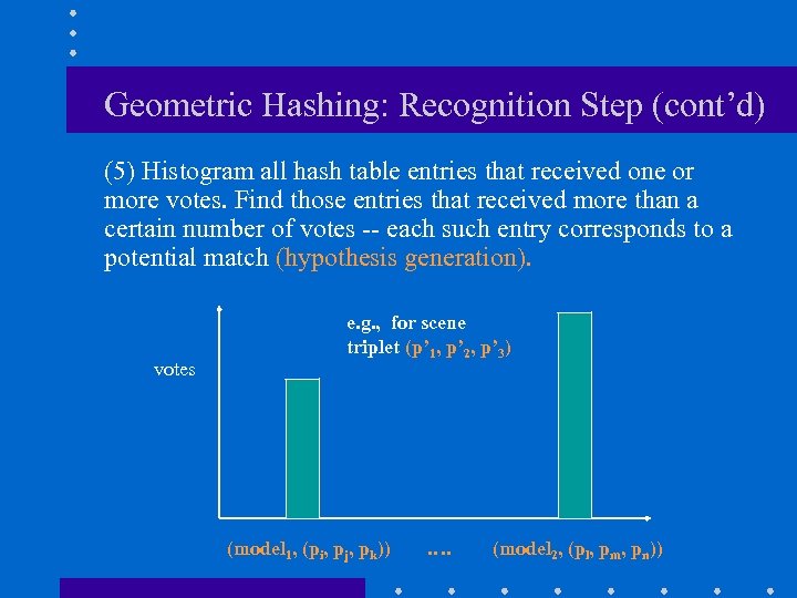
Geometric Hashing: Recognition Step (cont’d) (5) Histogram all hash table entries that received one or more votes. Find those entries that received more than a certain number of votes -- each such entry corresponds to a potential match (hypothesis generation). e. g. , for scene triplet (p’ 1, p’ 2, p’ 3) votes (model 1, (pi, pj, pk)) …. (model 2, (pl, pm, pn))

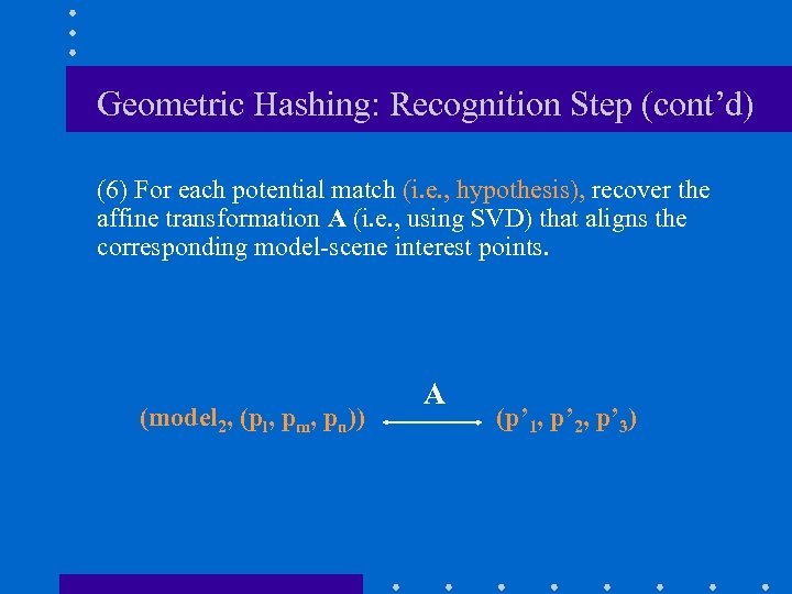
Geometric Hashing: Recognition Step (cont’d) (6) For each potential match (i. e. , hypothesis), recover the affine transformation A (i. e. , using SVD) that aligns the corresponding model-scene interest points. (model 2, (pl, pm, pn)) A (p’ 1, p’ 2, p’ 3)

Geometric Hashing: Recognition Step (cont’d) (7) Back-project the model onto the scene using the computed transform and compare the model with the scene to find additional matches (verification step). (8) If verification fails for all hypotheses step (5), go back to step (2) and repeat the procedure using a different group of scene features.

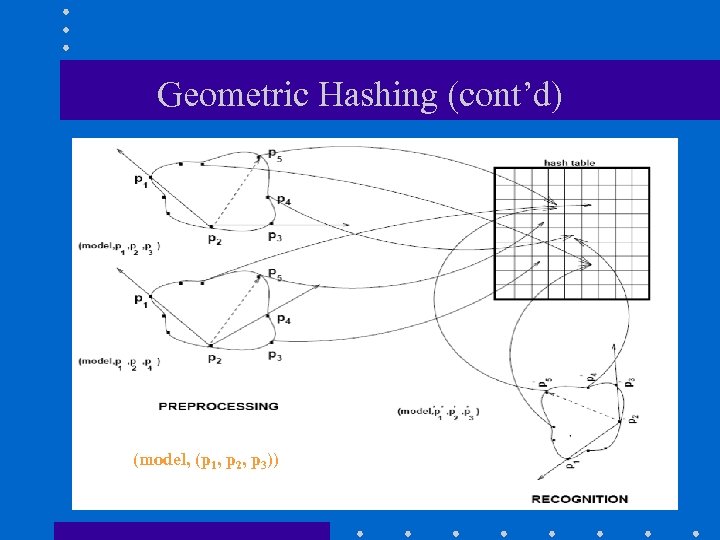
Geometric Hashing (cont’d) (model, (p 1, p 2, p 3))

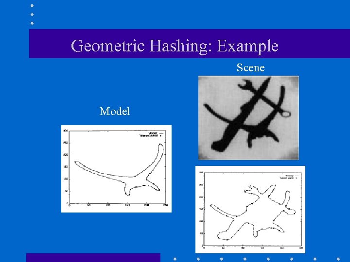
Geometric Hashing: Example Scene Model

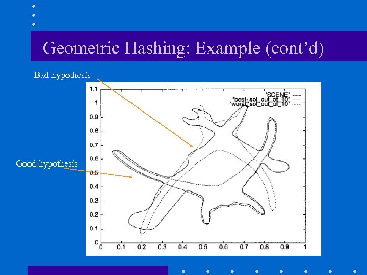
Geometric Hashing: Example (cont’d) Bad hypothesis Good hypothesis

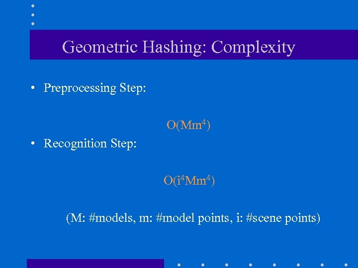
Geometric Hashing: Complexity • Preprocessing Step: O(Mm 4) • Recognition Step: O(i 4 Mm 4) (M: #models, m: #model points, i: #scene points)

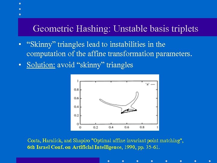
Geometric Hashing: Unstable basis triplets • “Skinny” triangles lead to instabilities in the computation of the affine transformation parameters. • Solution: avoid “skinny” triangles Costa, Haralick, and Shapiro "Optimal affine invariant point matching", 6 th Israel Conf. on Artificial Intelligence, 1990, pp. 35 -61.

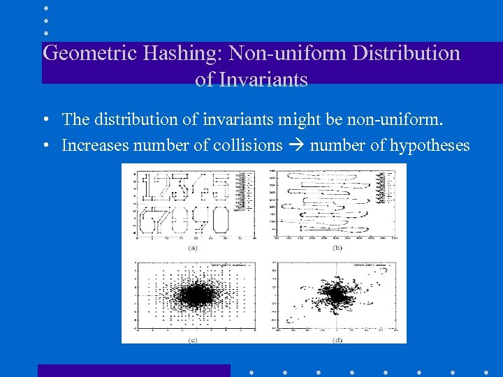
Geometric Hashing: Non-uniform Distribution of Invariants • The distribution of invariants might be non-uniform. • Increases number of collisions number of hypotheses

Geometric Hashing: Non-uniform Distribution of Invariants (cont’d) • Rehashing – Map the distribution of invariants to a uniform distribution. – Need to make assumptions about the distribution of invariants. I. Rigoutsos and R. Hummel, “Several Results on Affine Invariant Geometric Hashing, 8 th Israeli Conf on Artificial Intell. And Comp. Vision, 1991. • “Learn” geometric hash functions G. Bebis et al. , "Using Self-Organizing Maps to Learn Geometric Hashing Functions for Model-Based Object Recognition" , IEEE Transactions on Neural Networks, vol 9, no. 3, pp. 560 -570, 1998.

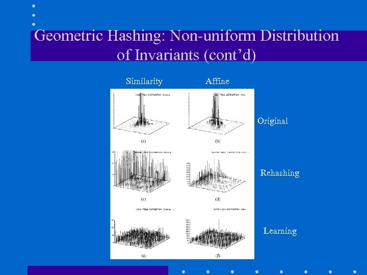
Geometric Hashing: Non-uniform Distribution of Invariants (cont’d) Similarity Affine Original Rehashing Learning

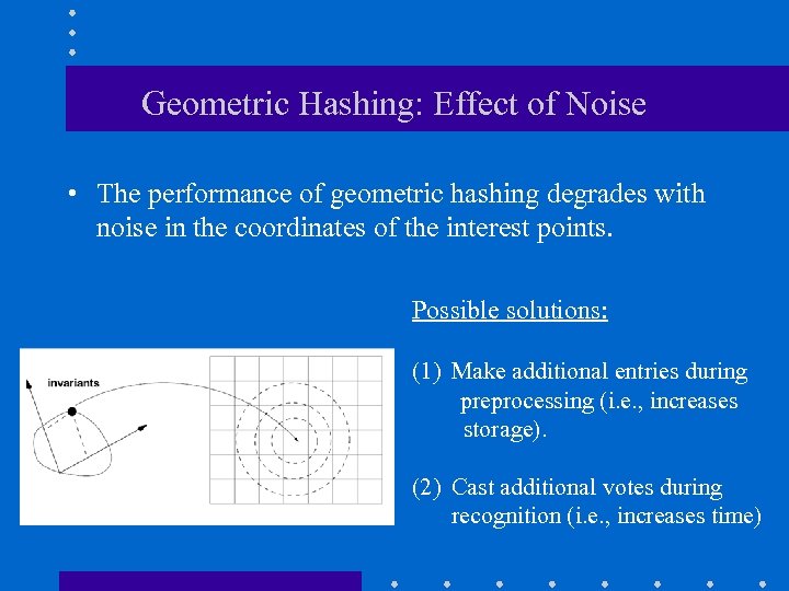
Geometric Hashing: Effect of Noise • The performance of geometric hashing degrades with noise in the coordinates of the interest points. Possible solutions: (1) Make additional entries during preprocessing (i. e. , increases storage). (2) Cast additional votes during recognition (i. e. , increases time)

Index Selectivity • Recognition accuracy could be improved by increasing index selectivity. – e. g. , using higher-dimensional indices A. Califano and R. Mohan, “Multidimensional Indexing for Recognizing Visual Shapes”, IEEE Transactions on Pattern Analysis and Machine Intelligence, vol. 16, no. 4, pp. 373 – 392, 1994

Object Recognition using SIFT features 1. Match individual SIFT features from an image to a database of SIFT features from known objects (i. e. , find nearest neighbors). 2. Find clusters of SIFT features belonging to a single object (hypothesis generation).

Object Recognition using SIFT features 3. Estimate object pose (i. e. , recover the transformation that the model has undergone) using at least three matches. 4. Verify that additional features agree on object pose.

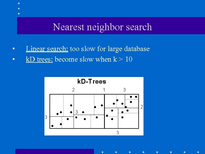
Nearest neighbor search • • Linear search: too slow for large database k. D trees: become slow when k > 10

Nearest neighbor search (cont’d) • Approximate nearest neighbor search: – – – • Best-bin-first [Beis et al. 97] (modification to k. D-tree algorithm) Examine only the N closest bins of the k. D-tree Use a heap to identify bins in order by their distance from query. Can give speedup by factor of 1000 while finding nearest neighbor (of interest) 95% of the time. FLANN - Fast Library for Approximate Nearest Neighbors Marius Muja and David G. Lowe, "Fast Approximate Nearest Neighbors with Automatic Algorithm Configuration", International Conference on Computer Vision Theory and Applications, 2009

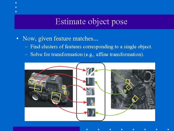
Estimate object pose • Now, given feature matches… – Find clusters of features corresponding to a single object. – Solve for transformation (e. g. , affine transformation).

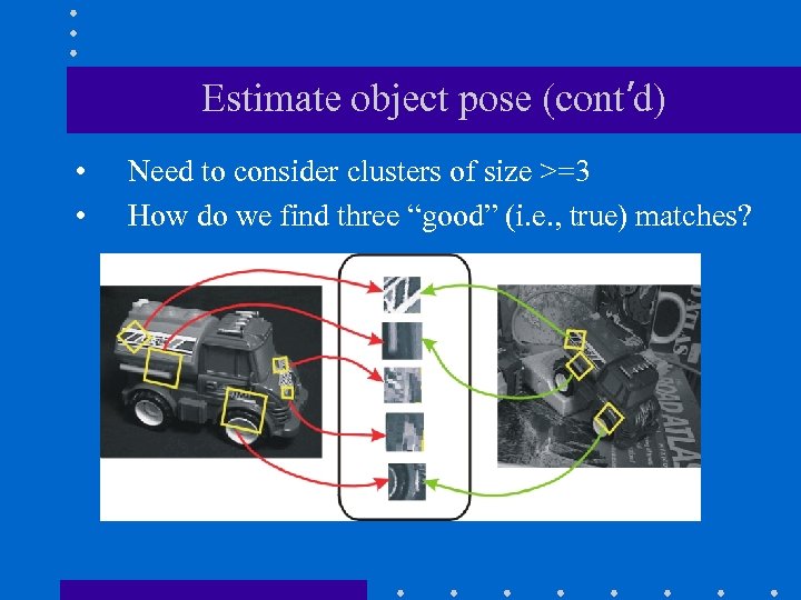
Estimate object pose (cont’d) • • Need to consider clusters of size >=3 How do we find three “good” (i. e. , true) matches?

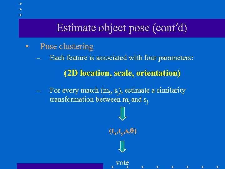
Estimate object pose (cont’d) • Pose clustering – Each feature is associated with four parameters: (2 D location, scale, orientation) – For every match (mi, sj), estimate a similarity transformation between mi and sj (tx, ty, s, θ) vote

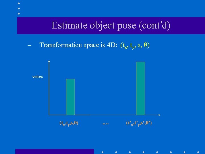
Estimate object pose (cont’d) – Transformation space is 4 D: (tx, ty, s, θ) votes (tx, ty, s, θ) …. (t’x, t’y, s’, θ’)

Estimate object pose (cont’d) – Partial voting: vote for neighboring bins and use large bin size to better tolerate errors. – Transformations that accumulate at least three votes are selected (hypothesis generation). – Using model-scene matches, compute object pose (i. e. , affine transformation) and apply verification.

Verification • Back-project model on the scene and look for additional matches. • Discard outliers (i. e. , incorrect matches) by imposing stricter matching constraints (e. g. , half error). • Find additional matches by refine the transformation computed (i. e. , iterative affine refinements).

Verification (cont’d) • Evaluate probability that match is correct. – Use Bayesian (probabilistic) model, to estimate the probability that a model is present based on the actual number of matching features. – Bayesian model takes into account: • • Object size in image Textured regions Model feature count in database Accuracy of fit Lowe, D. G. 2001. Local feature view clustering for 3 D object recognition. IEEE Conference on Computer Vision and Pattern Recognition, Kauai, Hawaii, pp. 682– 688.

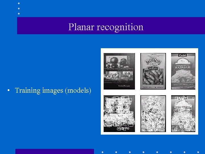
Planar recognition • Training images (models)

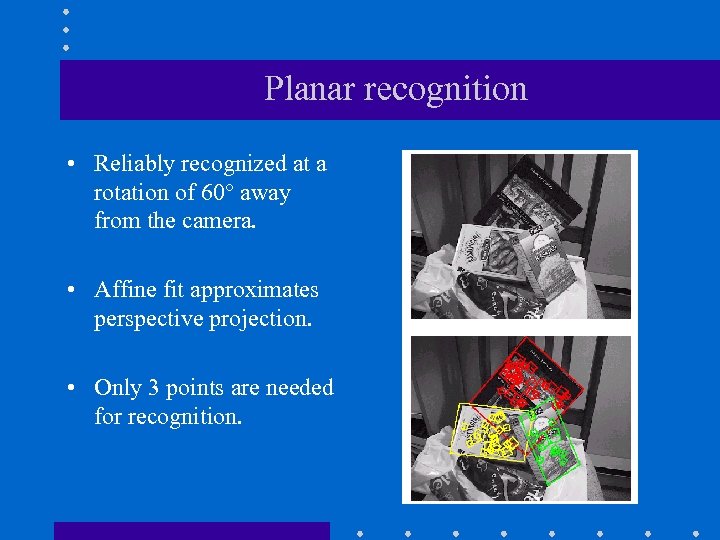
Planar recognition • Reliably recognized at a rotation of 60° away from the camera. • Affine fit approximates perspective projection. • Only 3 points are needed for recognition.

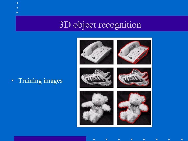
3 D object recognition • Training images

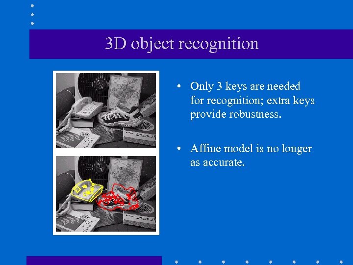
3 D object recognition • Only 3 keys are needed for recognition; extra keys provide robustness. • Affine model is no longer as accurate.

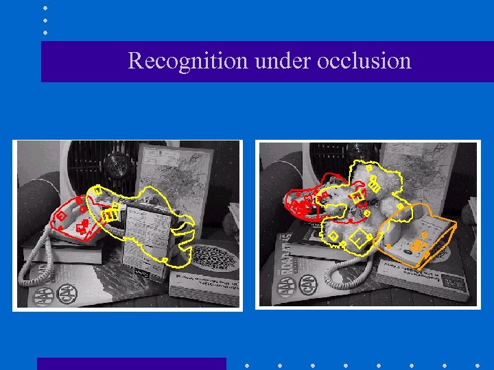
Recognition under occlusion

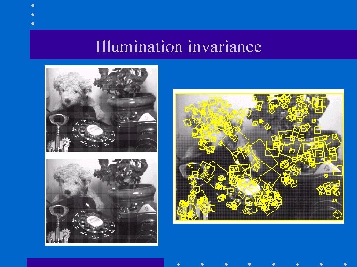
Illumination invariance

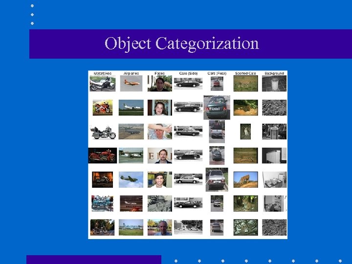
Object Categorization

Bag-of-features (Bo. F) models Good for object categorization

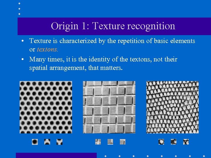
Origin 1: Texture recognition • Texture is characterized by the repetition of basic elements or textons. • Many times, it is the identity of the textons, not their spatial arrangement, that matters.

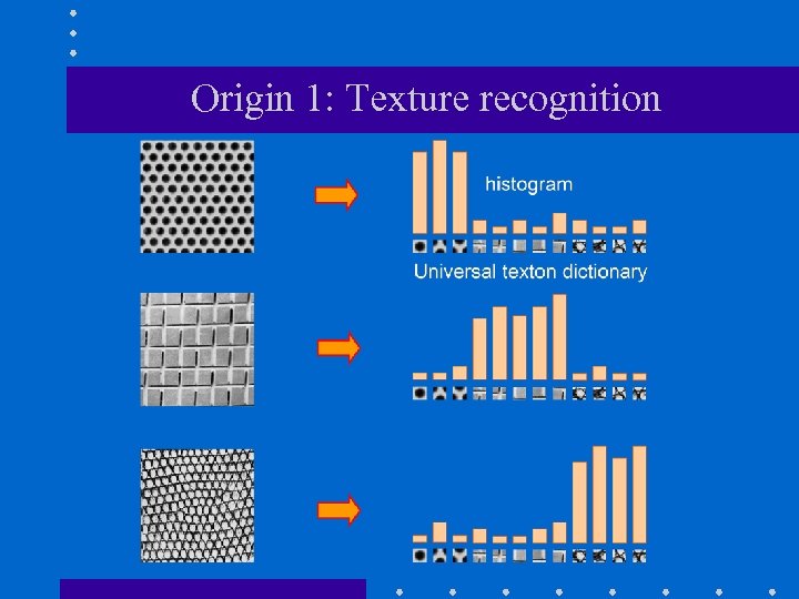
Origin 1: Texture recognition

Origin 2: Document retrieval • Orderless document representation: frequencies of words from a dictionary Salton & Mc. Gill (1983)

Bo. F for object categorization Need a “visual” dictionary! G. Cruska et al. , "Visual Categorization with Bags of Keypoints", European Conference on Computer Vision, Czech Republic, 2004

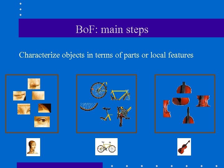
Bo. F: main steps Characterize objects in terms of parts or local features

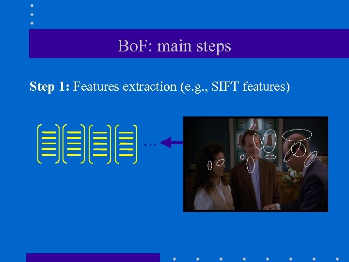
Bo. F: main steps Step 1: Features extraction (e. g. , SIFT features) …

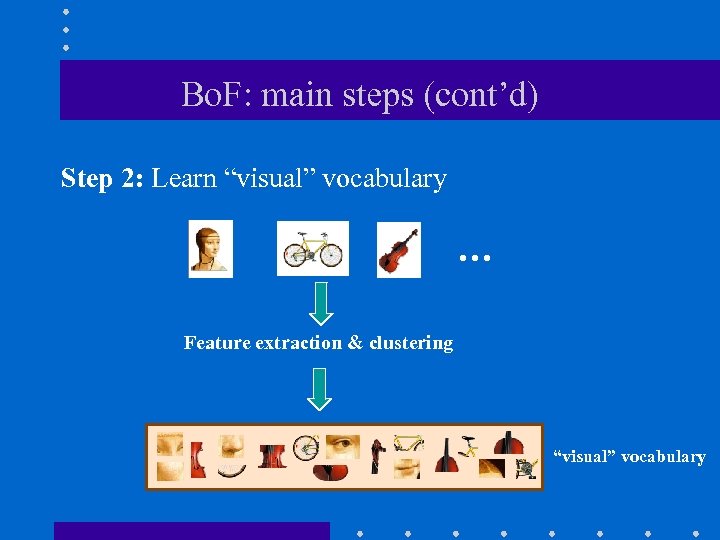
Bo. F: main steps (cont’d) Step 2: Learn “visual” vocabulary … Feature extraction & clustering “visual” vocabulary

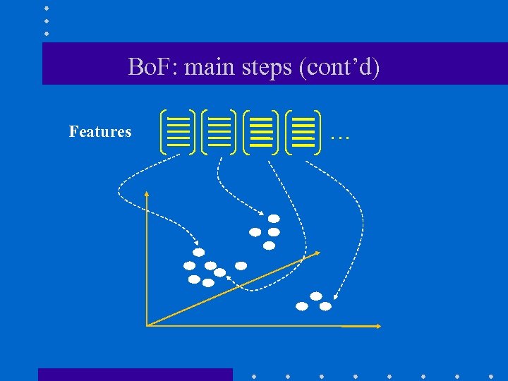
Bo. F: main steps (cont’d) Features …

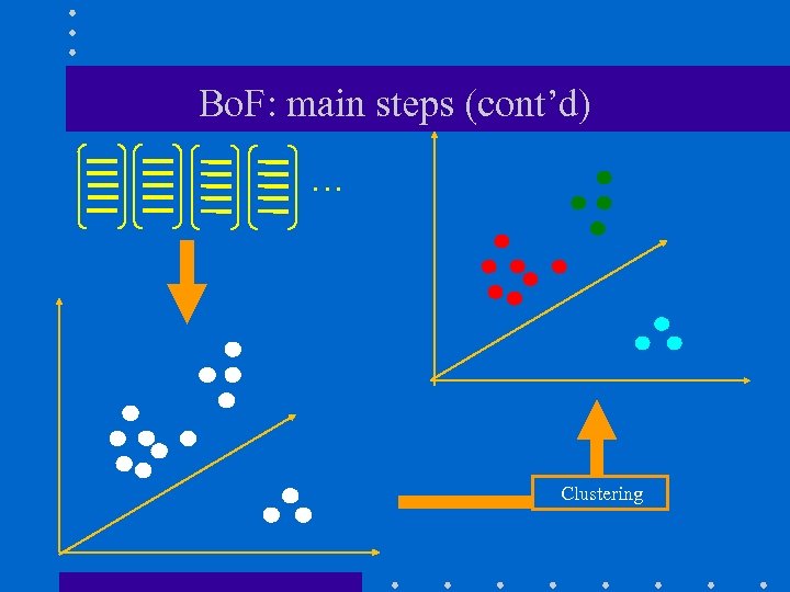
Bo. F: main steps (cont’d) … Clustering

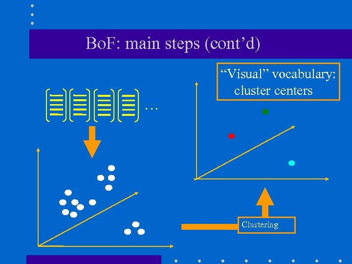
Bo. F: main steps (cont’d) … “Visual” vocabulary: cluster centers Clustering

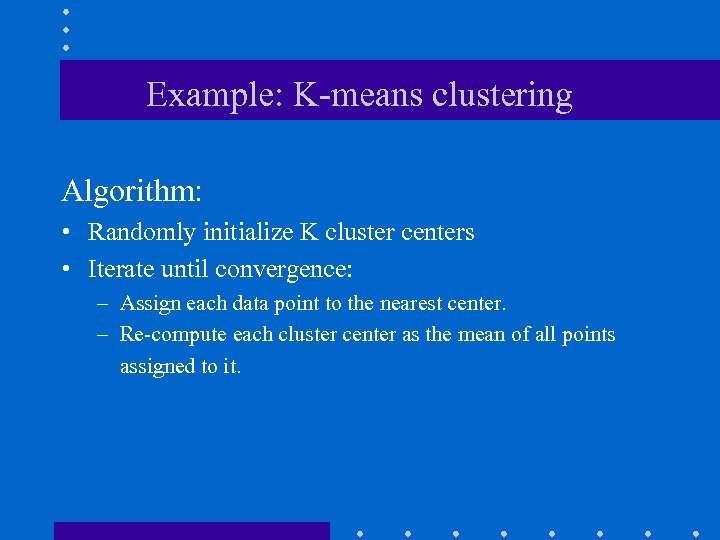
Example: K-means clustering Algorithm: • Randomly initialize K cluster centers • Iterate until convergence: – Assign each data point to the nearest center. – Re-compute each cluster center as the mean of all points assigned to it.

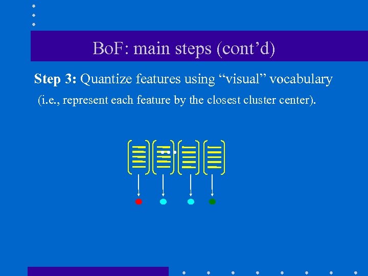
Bo. F: main steps (cont’d) Step 3: Quantize features using “visual” vocabulary (i. e. , represent each feature by the closest cluster center). …

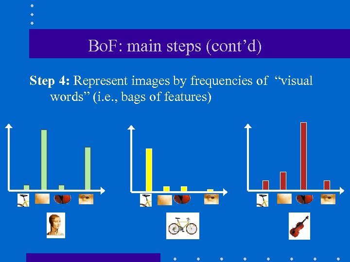
Bo. F: main steps (cont’d) Step 4: Represent images by frequencies of “visual words” (i. e. , bags of features)

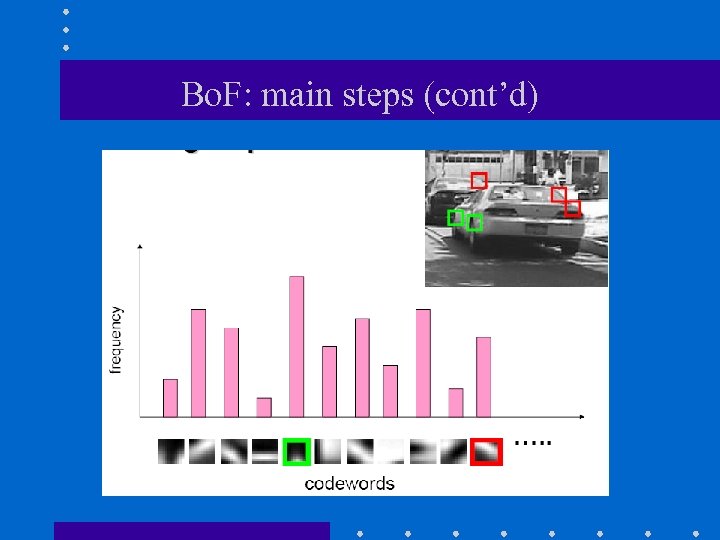
Bo. F: main steps (cont’d)

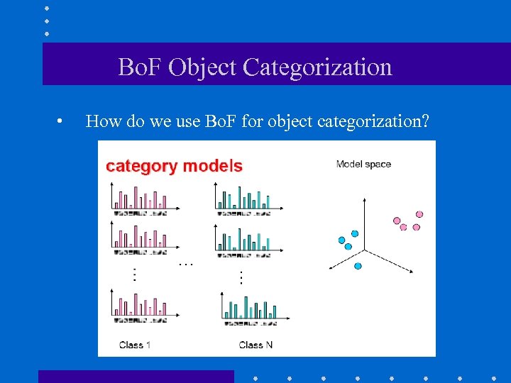
Bo. F Object Categorization • How do we use Bo. F for object categorization?

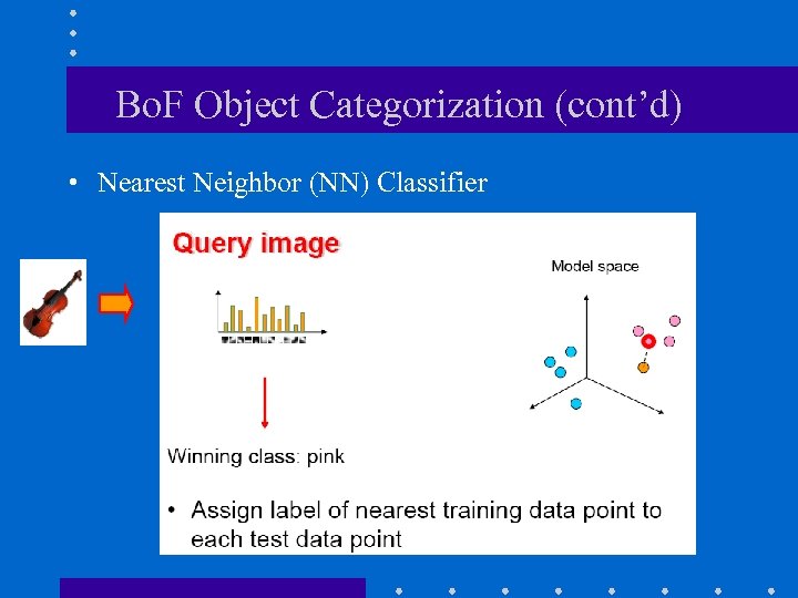
Bo. F Object Categorization (cont’d) • Nearest Neighbor (NN) Classifier

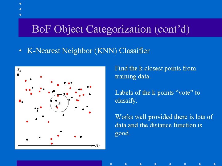
Bo. F Object Categorization (cont’d) • K-Nearest Neighbor (KNN) Classifier Find the k closest points from training data. Labels of the k points “vote” to classify. Works well provided there is lots of data and the distance function is good.

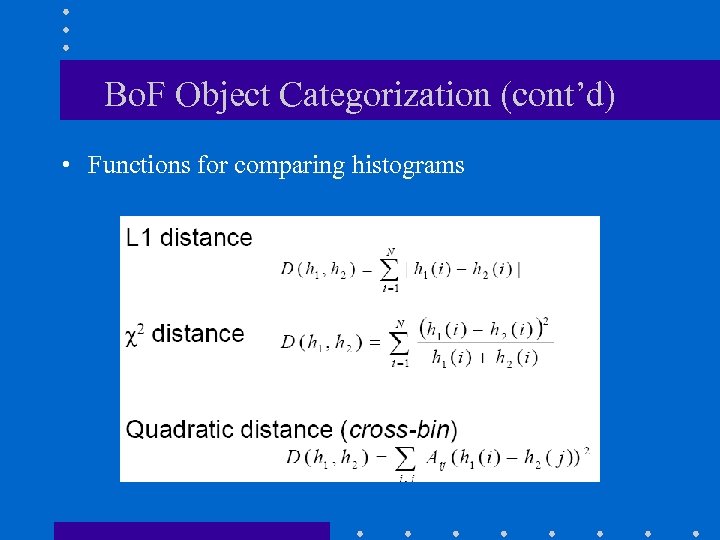
Bo. F Object Categorization (cont’d) • Functions for comparing histograms

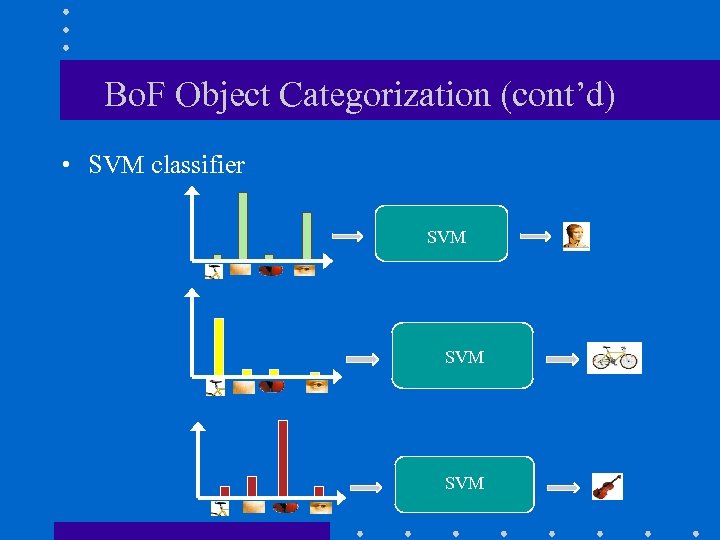
Bo. F Object Categorization (cont’d) • SVM classifier SVM

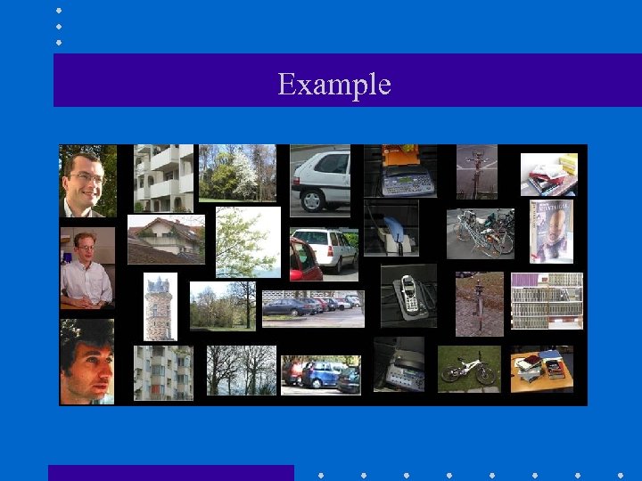
Example Caltech 6 dataset

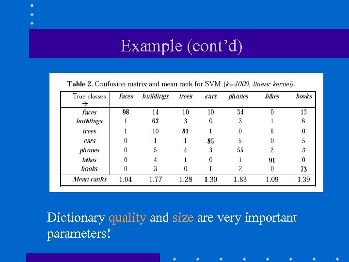
Example (cont’d) Caltech 6 dataset Dictionary quality and size are very important parameters!

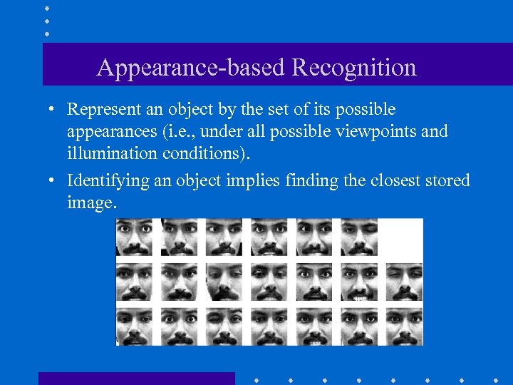
Appearance-based Recognition • Represent an object by the set of its possible appearances (i. e. , under all possible viewpoints and illumination conditions). • Identifying an object implies finding the closest stored image.

Appearance-based Recognition (cont’d) • In practice, a subset of all possible appearances is used. • Images are highly correlated, so “compress” them into a low-dimensional space that captures key appearance characteristics (e. g. , use Principal Component Analysis (PCA)). M. Turk and A. Pentland, Eigenfaces for Recognition, Journal of Cognitive Neuroscience, vol. 3, no. 1, pp. 71 -86, 1991. H. Murase and S. Nayar, Visual Learning and Recognition of 3 D Objects from Appearance, International Journal of Computer Vision, vol 14, pp. 5 -24, 1995.