NUMERICAL MODELING OF THE OCEAN AND MARINE DYNAMICS

NUMERICAL MODELING OF THE OCEAN AND MARINE DYNAMICS ON THE BASE OF MULTICOMPONENT SPLITTING Marchuk G. I. , Kordzadze A. A. , Tamsalu R, Zalesny V. B. , Agoshkov V. I. , Bagno A. V. , Gusev A. V. , Diansky N. A. , Moshonkin S. N. Moscow, 2010

Contents • I. Splitting method is a methodological basis for the construction and treatment of the complicated system • II. Nonhydrostatic FRESCO model of the Baltic Sea • III. Numerical model of the Black Sea dynamics • IV. World Ocean -coordinate splitting model • V. 4 D VAR data assimilation techniques based on splitting and adjoint equation methods

I. Splitting method is a methodological basis for the construction and treatment of the complicated hydro-ecosystem. Key points • The splitting method can be considered not only as a costeffective solution of the complex problem but as the basis for the construction of the hierarchical model system as well • In the framework of the unified approach there can be constructed a particular model of sea/ocean dynamics of a different complexity: from the point of view of its physical completeness, dimension, and spatial resolution • We need to find a conservation law which holds in the model in the absence of external sources and internal energy sinks

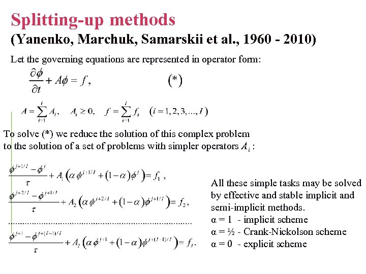Splitting-up methods (Yanenko, Marchuk, Samarskii et al. , 1960 - 2010) Let the governing equations are represented in operator form: To solve (*) we reduce the solution of this complex problem to the solution of a set of problems with simpler operators Ai : All these simple tasks may be solved by effective and stable implicit and semi-implicit methods. α = 1 - implicit scheme α = ½ - Crank-Nickolson scheme α = 0 - explicit scheme

Multicomponent splitting • Symmetrized form of governing equations • Energy conserving space approximations using V. I. Lebedev grids • Multicomponent splitting into series of nonnegative subproblems • Separate subproblem has its adjoint analog. The adjoint model consists of the respective subsystems adjoint to the split subsystems of the forward model • Implicit schemes and exact solutions

II. Nonhydrostatic FRESCO numerical model (Tamsalu et al. ) • The goal of experiments is to simulate the dynamics of the Baltic Sea in an eddying regime • Experiments are carried out for four nested regions with a gradual improvement of the spatial resolution: the Baltic Sea (h = 3. 7 km), Gulf of Finland ( h = 1. 85 km), Tallinn. Helsinki basin ( h=460 m ), Tallinn Bay (h = 93 m). Atmospheric forcing: HIRLAM forecast for August 2003 • The model simulates the processes of enhanced turbulence activity in the near-shore zones

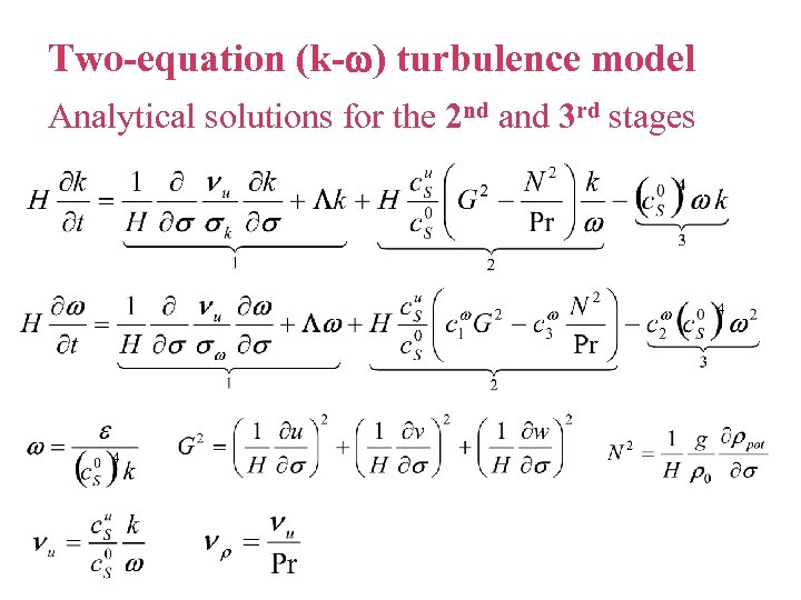Two-equation (k- ) turbulence model Analytical solutions for the 2 nd and 3 rd stages

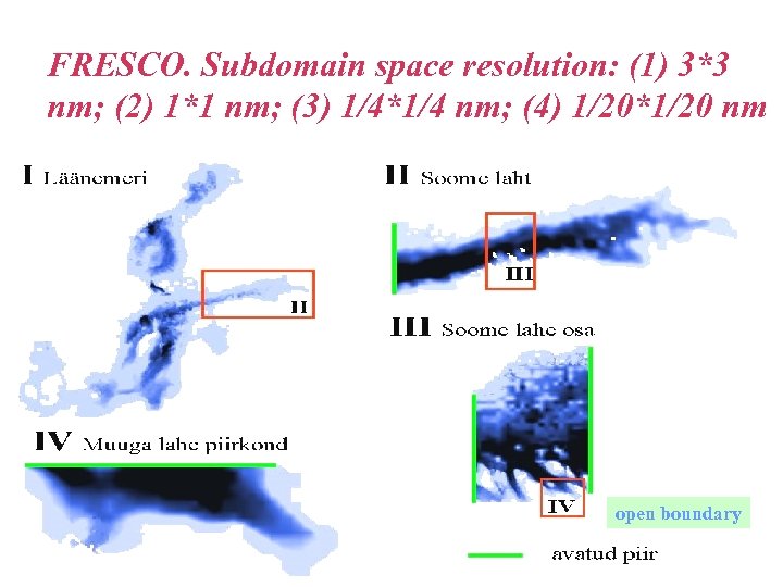FRESCO. Subdomain space resolution: (1) 3*3 nm; (2) 1*1 nm; (3) 1/4*1/4 nm; (4) 1/20*1/20 nm open boundary

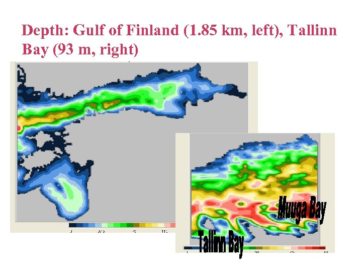Depth: Gulf of Finland (1. 85 km, left), Tallinn Bay (93 m, right)

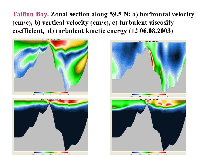Tallinn Bay. Zonal section along 59. 5 N: a) horizontal velocity (cm/c), b) vertical velocity (cm/c), c) turbulent viscosity coefficient, d) turbulent kinetic energy (12 06. 08. 2003)

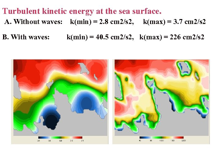Turbulent kinetic energy at the sea surface. A. Without waves: B. With waves: k(min) = 2. 8 cm 2/s 2, k(max) = 3. 7 cm 2/s 2 k(min) = 40. 5 cm 2/s 2, k(max) = 226 cm 2/s 2

III. Mathematical modeling of the Black Sea dynamics Institute of Geophysics, Georgia, Tbilisi (A. Kordzadze et al. ) • Primitive equation model. Splitting numerical technique • Splitting with respect to (x, z) and (y, z) plans • 5 -10 km resolution for the most part of the Black Sea • 1 km resolution of the Eastern Black Sea (from 39. 32 E): 216 x 347 x 30 • Forecast duration: 4 days. . . initial cond. from MHI (Sebastopol), atmospheric forecast fields at 1 hour intervals from ALADIN atmospheric model

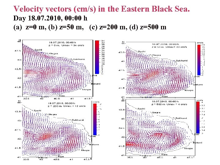Velocity vectors (cm/s) in the Eastern Black Sea. Day 18. 07. 2010, 00: 00 h (a) z=0 m, (b) z=50 m, (c) z=200 m, (d) z=500 m

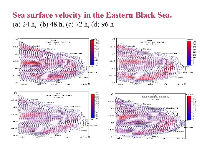Sea surface velocity in the Eastern Black Sea. (a) 24 h, (b) 48 h, (c) 72 h, (d) 96 h

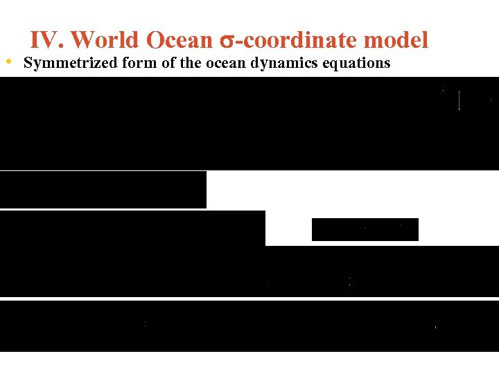IV. World Ocean -coordinate model • Symmetrized form of the ocean dynamics equations

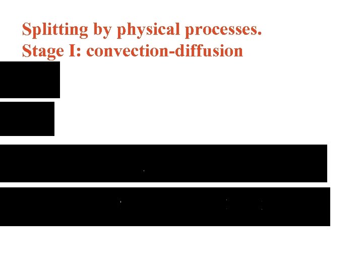Splitting by physical processes. Stage I: convection-diffusion

Splitting by physical processes. Stage II: adaptation of density and velocity fields

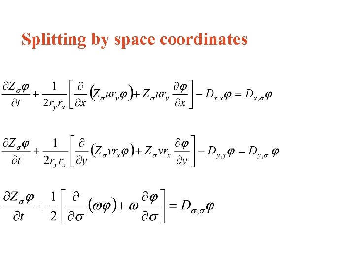Splitting by space coordinates

V. 4 D-var data assimilation technique (Marchuk, Penenko, Le Dimet, Talagrand, Agoshkov, Shutyaev et al. , 1978 – 2010) • 4 D-Var data assimilation method is applied in • • oceanography to solve inverse problems It is used to find a set of control variables, which minimize the norm of distance between observations and model predictions (cost function) Using adjoint equation method the gradient of the cost function is computed and optimal control method is implemented to solve problems arising in ocean modeling

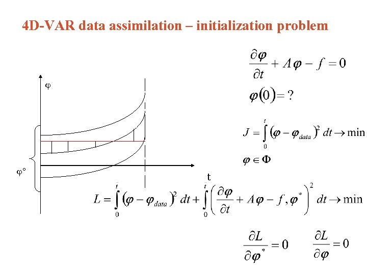4 D-VAR data assimilation – initialization problem ° t

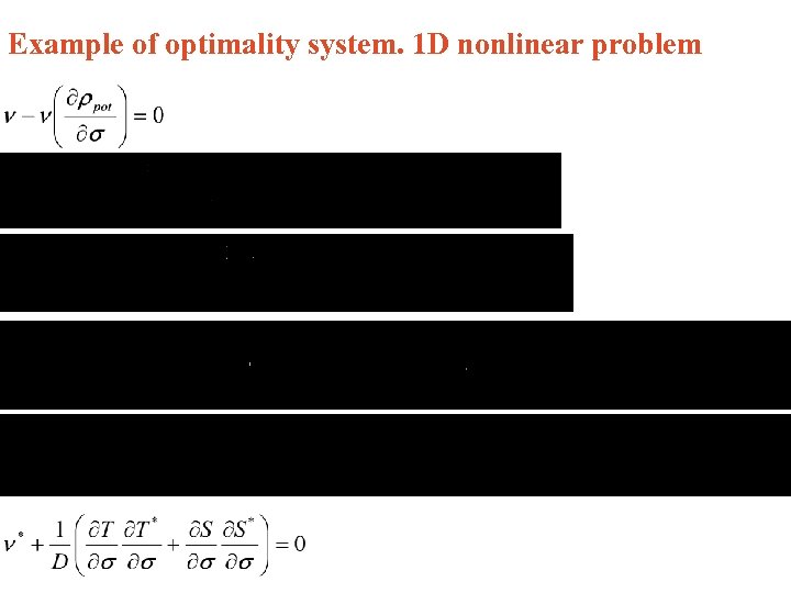Example of optimality system. 1 D nonlinear problem

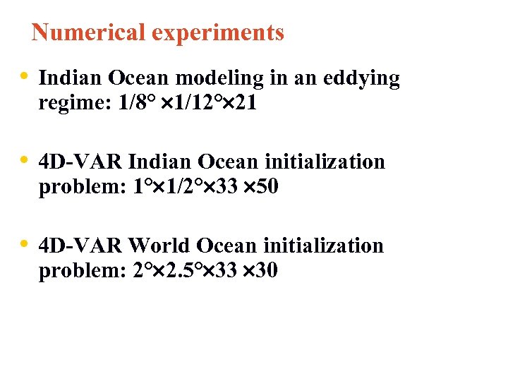Numerical experiments • Indian Ocean modeling in an eddying regime: 1/8° 1/12° 21 • 4 D-VAR Indian Ocean initialization problem: 1° 1/2° 33 50 • 4 D-VAR World Ocean initialization problem: 2° 2. 5° 33 30

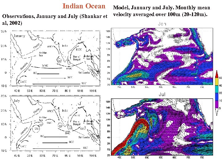Indian Ocean Observations, January and July (Shankar et al, 2002) Model, January and July. Monthly mean velocity averaged over 100 m (20 -120 m).

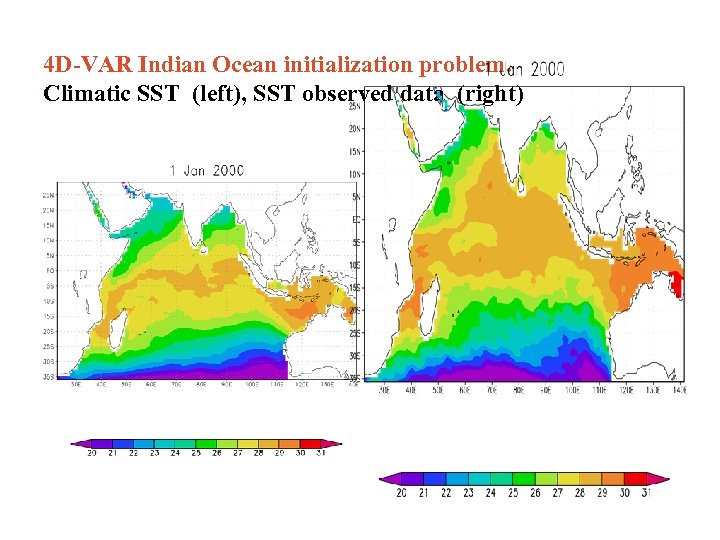4 D-VAR Indian Ocean initialization problem. Climatic SST (left), SST observed data (right)

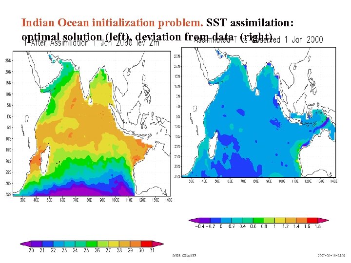Indian Ocean initialization problem. SST assimilation: optimal solution (left), deviation from data (right)

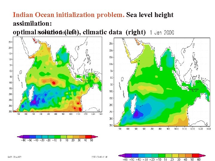Indian Ocean initialization problem. Sea level height assimilation: optimal solution (left), climatic data (right)

4 D-VAR World Ocean initialization problem • Two stages for the numerical experiments: climatic run and 4 D-VAR initialization of temperature and salinity fields • First stage: the World Ocean circulation under climatological atmospheric forcing (~ 3000 years) • Second stage: 4 D-VAR initialization of temperature and salinity fields using ARGO data (Zakharova, 2009). 5 -day assimilation interval, every month, 1 year.

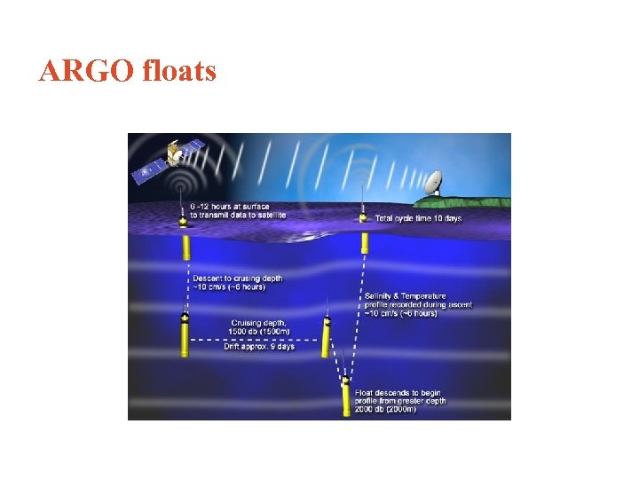ARGO floats Буи АРГО

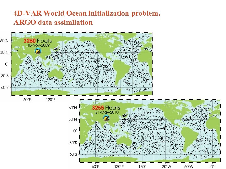4 D-VAR World Ocean initialization problem. ARGO data assimilation

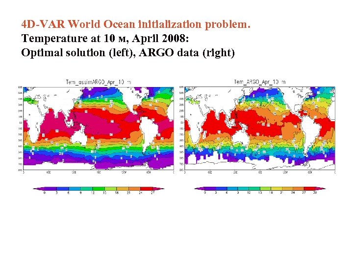4 D-VAR World Ocean initialization problem. Temperature at 10 м, April 2008: Optimal solution (left), ARGO data (right)

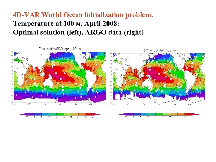4 D-VAR World Ocean initialization problem. Temperature at 100 м, April 2008: Optimal solution (left), ARGO data (right)

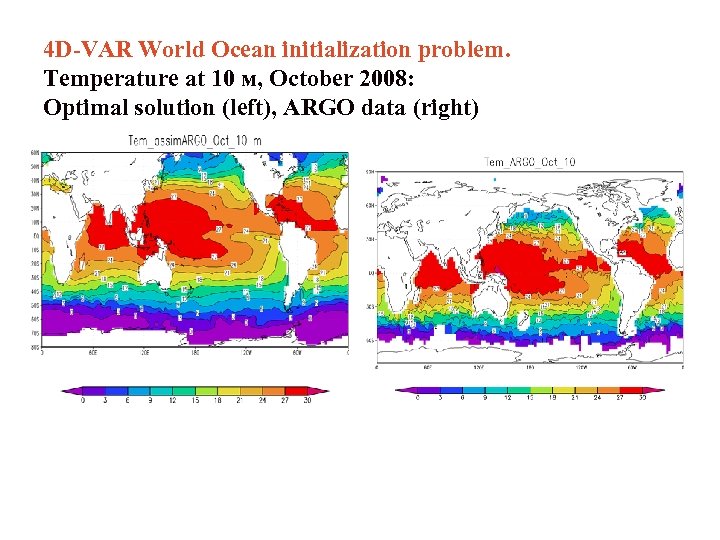4 D-VAR World Ocean initialization problem. Temperature at 10 м, October 2008: Optimal solution (left), ARGO data (right)

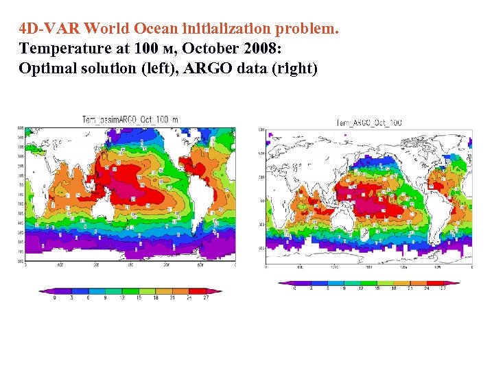4 D-VAR World Ocean initialization problem. Temperature at 100 м, October 2008: Optimal solution (left), ARGO data (right)

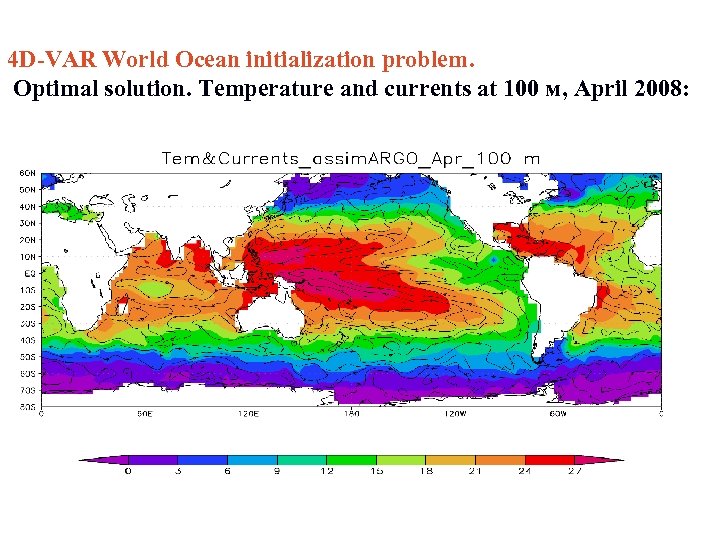4 D-VAR World Ocean initialization problem. Optimal solution. Temperature and currents at 100 м, April 2008:

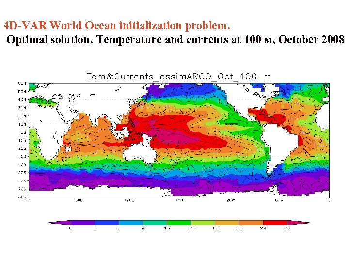4 D-VAR World Ocean initialization problem. Optimal solution. Temperature and currents at 100 м, October 2008

Conclusions • Splitting numerical technique for the solution of the prognostic and 4 D-VAR ocean data assimilation problem is constructed • As a result of splitting, a rather simple subsystems of the forward and adjoint equations are solved at each separate stage • Adjoint model consists of the respective subsystems adjoint to the split subsystems of the forward model • The method is the constructive basis for the INM modular computing system of simulation and initialization of the World Ocean hydrographic fields

To split or not to split?