1e5672a658e698ac5ce80f06d577bbd7.ppt
- Количество слайдов: 23
 Numerical Descriptive Measures 1
 Motivation • What is the “average consumer” exactly? • Why is it that if an average yield on an investment (e. g. mutual fund) is 28% that I’ve lost money? • At Morning Brew people arrive on average 1 per min and it takes typically 1 min to serve them, why is it that if I staff the register with 1 person people complain that the lines are too long and often leave before purchasing something? • If I plan our payables based on an average daily receivables of $7, 000 why have I gone bankrupt? • Why do students always want to know what the average on the exam was? 2
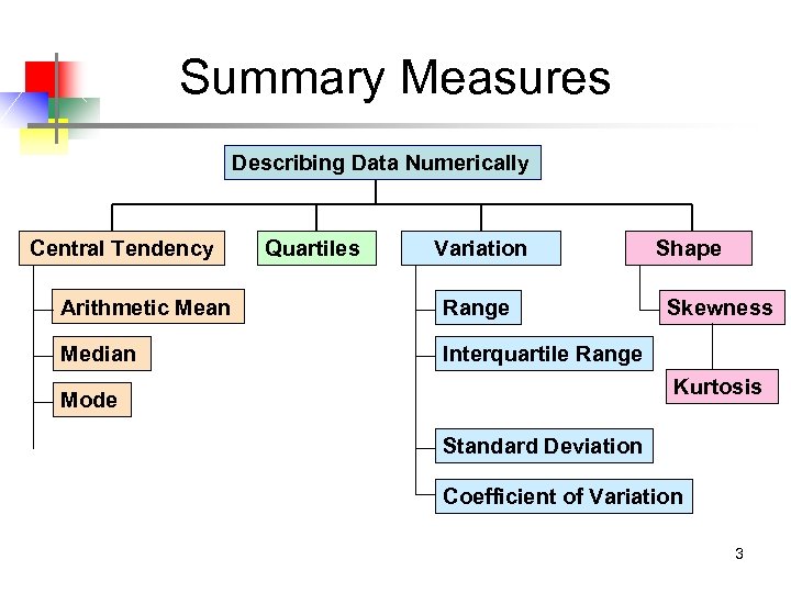 Summary Measures Describing Data Numerically Central Tendency Quartiles Variation Arithmetic Mean Range Median Shape Interquartile Range Skewness Kurtosis Mode Standard Deviation Coefficient of Variation 3
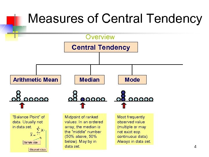 Measures of Central Tendency Overview Central Tendency Arithmetic Mean “Balance Point” of data. Usually not in data set. Median Midpoint of ranked values. In an ordered array, the median is the “middle” number (50% above, 50% below). May by in data set. Mode Most frequently observed value (multiple or may not exist esp. continuous data). Always in data set. 4
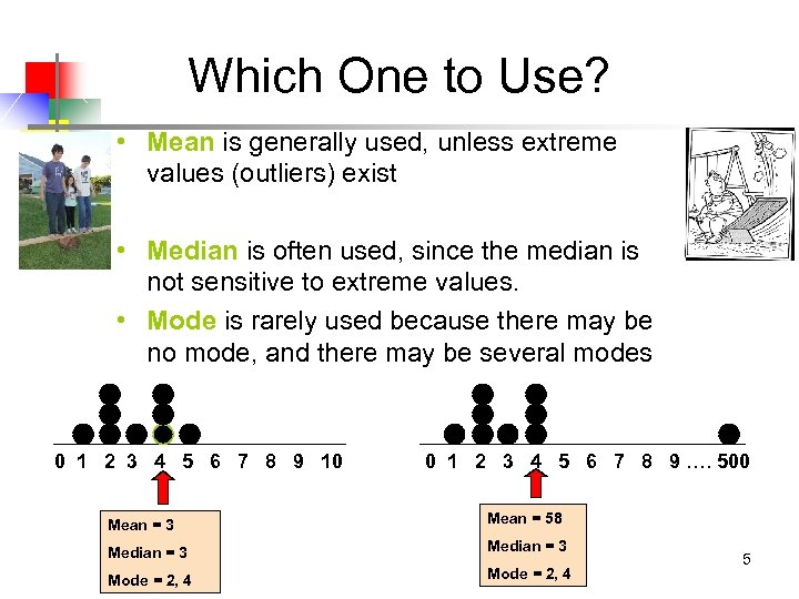 Which One to Use? • Mean is generally used, unless extreme values (outliers) exist • Median is often used, since the median is not sensitive to extreme values. • Mode is rarely used because there may be no mode, and there may be several modes 0 1 2 3 4 5 6 7 8 9 10 0 1 2 3 4 5 6 7 8 9 …. 500 Mean = 3 Mean = 58 Median = 3 Mode = 2, 4 5
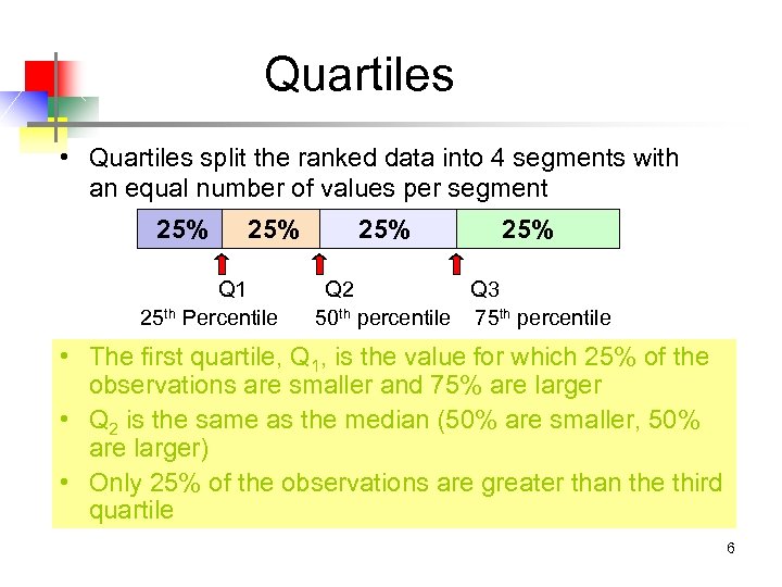 Quartiles • Quartiles split the ranked data into 4 segments with an equal number of values per segment 25% Q 1 25 th Percentile 25% Q 2 Q 3 50 th percentile 75 th percentile • The first quartile, Q 1, is the value for which 25% of the observations are smaller and 75% are larger • Q 2 is the same as the median (50% are smaller, 50% are larger) • Only 25% of the observations are greater than the third quartile 6
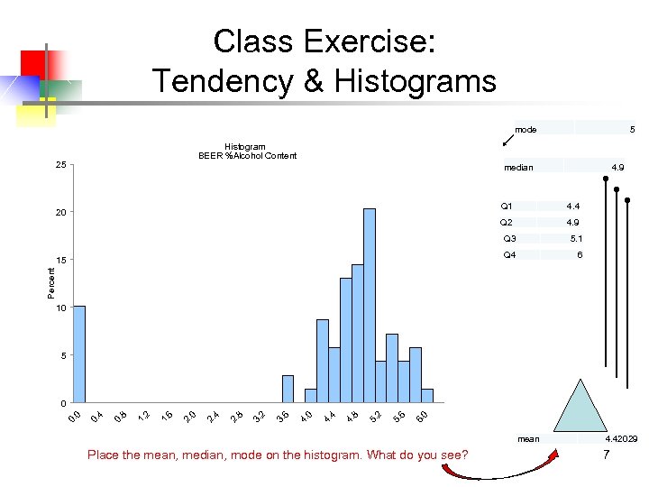 Class Exercise: Tendency & Histograms mode 5 Histogram BEER %Alcohol Content 25 median 4. 9 Q 1 4. 4 Q 2 20 4. 9 Q 3 Q 4 6 Percent 15 5. 1 10 5 0 6. 6 5. 2 5. 8 4. 4 4. 0 4. 6 3. 2 3. 8 2. 4 2. 0 2. 6 1. 2 1. 8 0. 4 0. 0 0 mean Place the mean, median, mode on the histogram. What do you see? 4. 42029 7
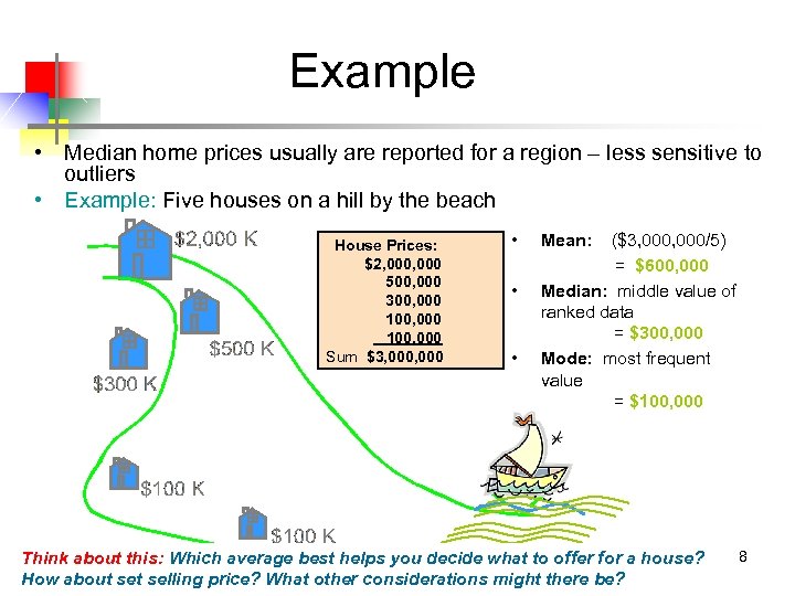 Example • Median home prices usually are reported for a region – less sensitive to outliers • Example: Five houses on a hill by the beach House Prices: $2, 000 500, 000 300, 000 100, 000 Sum $3, 000 • • • Mean: ($3, 000/5) = $600, 000 Median: middle value of ranked data = $300, 000 Mode: most frequent value = $100, 000 Think about this: Which average best helps you decide what to offer for a house? How about selling price? What other considerations might there be? 8
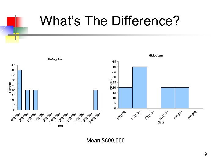 00 00 0, 0 75 00 0, 0 70 00 0, 0 0 65 5 00 10 0, 0 15 60 20 00 25 0, 0 35 55 40 00 30 Percent 45 0, 0 Percent Histogram 50 0, 00 1, 10 0 0, 00 1, 30 0 0, 00 1, 50 0 0, 00 1, 70 0 0, 00 1, 90 0 0, 00 2, 10 0 0, 00 0 90 00 0, 0 70 0, 0 50 00 00 0, 0 30 0, 0 10 What’s The Difference? Histogram 45 40 35 30 25 20 15 10 5 0 Data Mean $600, 000 9
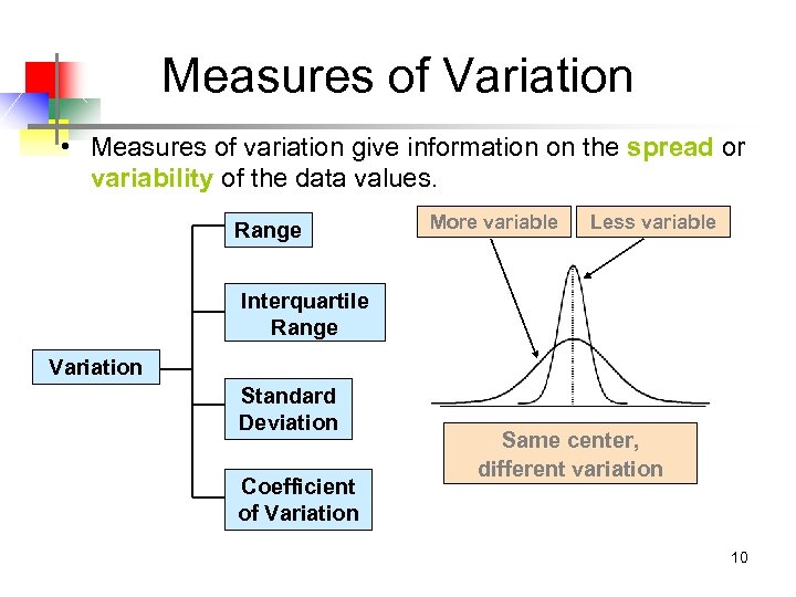 Measures of Variation • Measures of variation give information on the spread or variability of the data values. Range More variable Less variable Interquartile Range Variation Standard Deviation Coefficient of Variation Same center, different variation 10
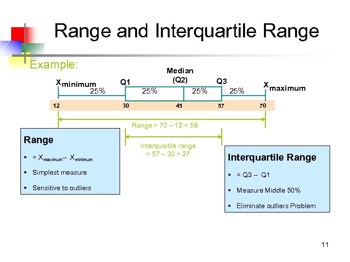 Range and Interquartile Range Example: X minimum 25% 12 Q 1 25% 30 Median (Q 2) 25% 45 Q 3 25% 57 X maximum 70 Range = 70 – 12 = 58 Range § = Xmaximum– Xminimum Interquartile range = 57 – 30 = 27 Interquartile Range § Simplest measure § = Q 3 – Q 1 § Sensitive to outliers § Measure Middle 50% § Eliminate outliers Problem 11
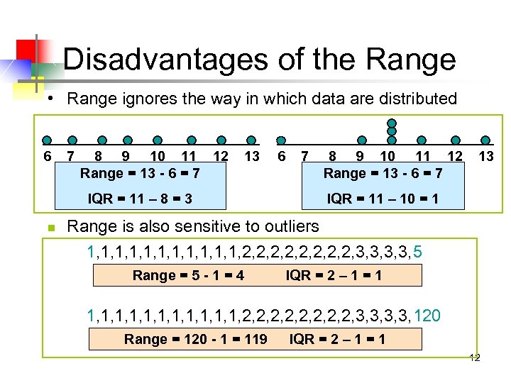 Disadvantages of the Range • Range ignores the way in which data are distributed 6 7 8 9 10 11 12 Range = 13 - 6 = 7 13 IQR = 11 – 8 = 3 n 6 7 8 9 10 11 12 Range = 13 - 6 = 7 13 IQR = 11 – 10 = 1 Range is also sensitive to outliers 1, 1, 1, 2, 2, 3, 3, 5 Range = 5 - 1 = 4 IQR = 2 – 1 = 1 1, 1, 1, 2, 2, 3, 3, 120 Range = 120 - 1 = 119 IQR = 2 – 1 = 1 12
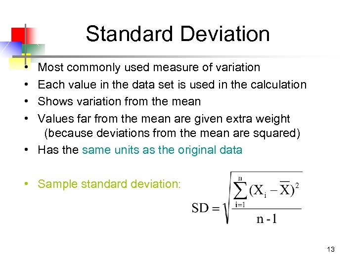 Standard Deviation • • Most commonly used measure of variation Each value in the data set is used in the calculation Shows variation from the mean Values far from the mean are given extra weight (because deviations from the mean are squared) • Has the same units as the original data • Sample standard deviation: 13
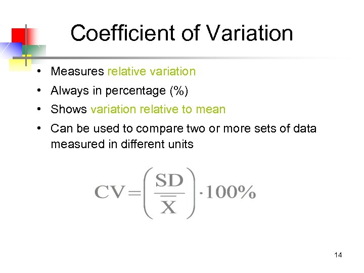 Coefficient of Variation • Measures relative variation • Always in percentage (%) • Shows variation relative to mean • Can be used to compare two or more sets of data measured in different units 14
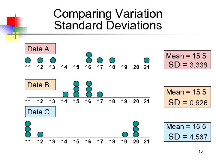 Comparing Variation Standard Deviations Data A 11 12 13 14 15 16 17 18 19 20 21 Mean = 15. 5 SD = 3. 338 20 21 Mean = 15. 5 SD = 0. 926 Data B 11 12 13 14 15 16 17 18 19 Data C 11 12 13 14 15 16 17 18 19 20 21 Mean = 15. 5 SD = 4. 567 15
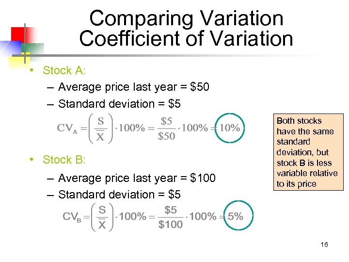 Comparing Variation Coefficient of Variation • Stock A: – Average price last year = $50 – Standard deviation = $5 • Stock B: – Average price last year = $100 – Standard deviation = $5 Both stocks have the same standard deviation, but stock B is less variable relative to its price 16
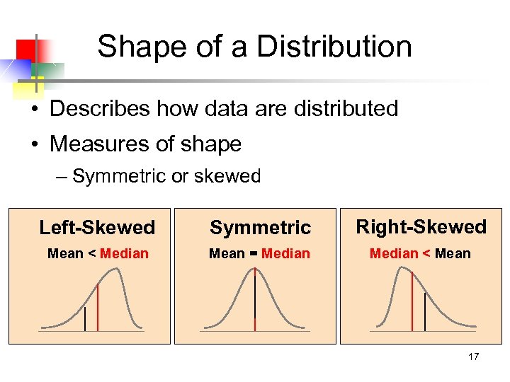 Shape of a Distribution • Describes how data are distributed • Measures of shape – Symmetric or skewed Left-Skewed Symmetric Right-Skewed Mean < Median Mean = Median < Mean 17
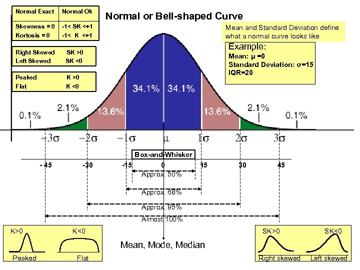 Normal Exact Normal Ok Skewness = 0 Kortosis = 0 -1< SK <+1 -1< K <+1 Right Skewed Left Skewed Mean and Standard Deviation define what a normal curve looks like Example: SK >0 SK <0 Peaked Flat Normal or Bell-shaped Curve K >0 K <0 Mean: μ =0 Standard Deviation: σ=15 IQR=20 Box-and-Whisker - 45 -30 -15 0 Approx. 50% 15 30 45 Approx. 68% Approx. 95% Almost 100% K>0 SK>0 K<0 Mean, Mode, Median Peaked Flat Right skewed SK<0 18 Left skewed
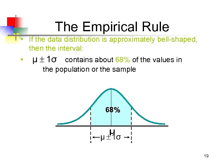 The Empirical Rule • If the data distribution is approximately bell-shaped, then the interval: • contains about 68% of the values in the population or the sample 68% 19
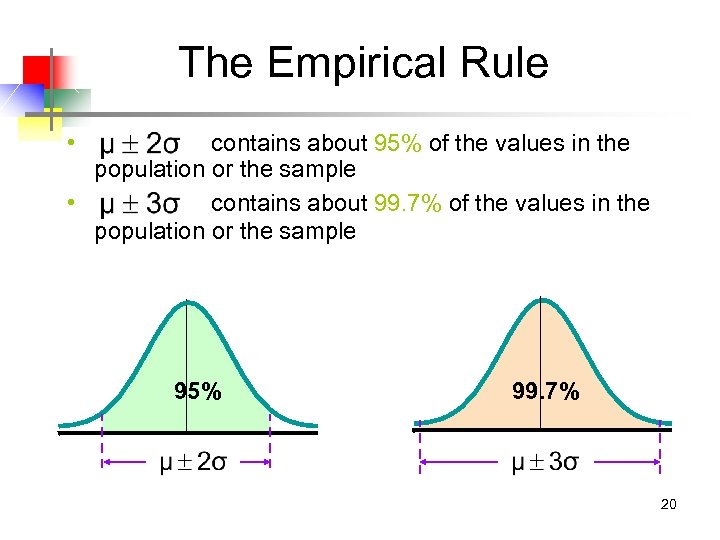 The Empirical Rule • contains about 95% of the values in the population or the sample • contains about 99. 7% of the values in the population or the sample 95% 99. 7% 20
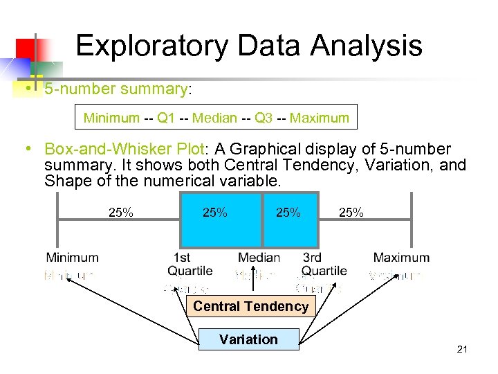 Exploratory Data Analysis • 5 -number summary: Minimum -- Q 1 -- Median -- Q 3 -- Maximum • Box-and-Whisker Plot: A Graphical display of 5 -number summary. It shows both Central Tendency, Variation, and Shape of the numerical variable. 25% 25% Central Tendency Variation 21
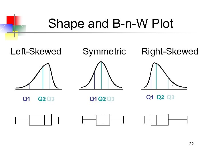 Shape and B-n-W Plot Left-Skewed Q 1 Q 2 Q 3 Symmetric Q 1 Q 2 Q 3 Right-Skewed Q 1 Q 2 Q 3 22
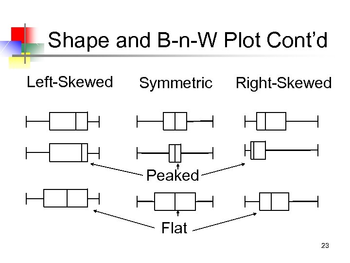 Shape and B-n-W Plot Cont’d Left-Skewed Symmetric Right-Skewed Peaked Flat 23


