Normalization for c DNA Microarray Data Yee Hwa

Normalization for c. DNA Microarray Data Yee Hwa Yang, Sandrine Dudoit, Percy Luu and Terry Speed. SPIE BIOS 2001, San Jose, CA January 22, 2001

Normalization issues Within-slide – What genes to use – Location – Scale Paired-slides (dye swap) – Self-normalization Between slides

Within-Slide Normalization —Normalization balances red and green intensities. —Imbalances can be caused by – Different incorporation of dyes – Different amounts of m. RNA – Different scanning parameters —In practice, we usually need to increase the red intensity a bit to balance the green

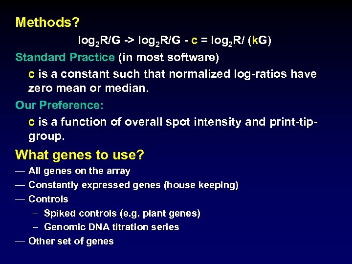Methods? log 2 R/G -> log 2 R/G - c = log 2 R/ (k. G) Standard Practice (in most software) c is a constant such that normalized log-ratios have zero mean or median. Our Preference: c is a function of overall spot intensity and print-tipgroup. What genes to use? — All genes on the array — Constantly expressed genes (house keeping) — Controls – Spiked controls (e. g. plant genes) – Genomic DNA titration series — Other set of genes

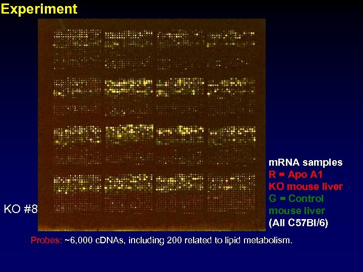Experiment KO #8 m. RNA samples R = Apo A 1 KO mouse liver G = Control mouse liver (All C 57 Bl/6) Probes: ~6, 000 c. DNAs, including 200 related to lipid metabolism.

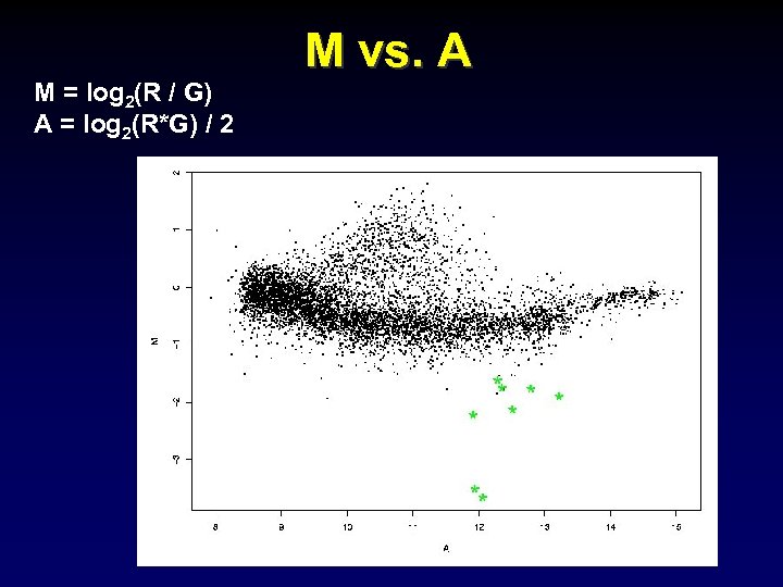M = log 2(R / G) A = log 2(R*G) / 2 M vs. A

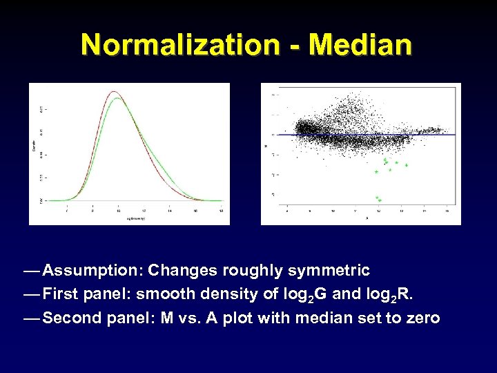Normalization - Median — Assumption: Changes roughly symmetric — First panel: smooth density of log 2 G and log 2 R. — Second panel: M vs. A plot with median set to zero

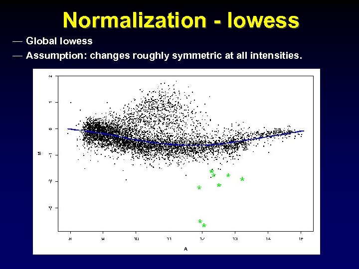Normalization - lowess — Global lowess — Assumption: changes roughly symmetric at all intensities.

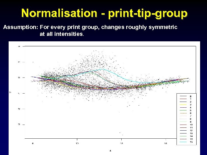Normalisation - print-tip-group Assumption: For every print group, changes roughly symmetric at all intensities.

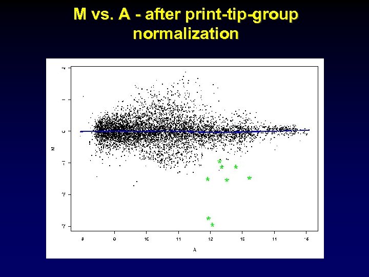M vs. A - after print-tip-group normalization

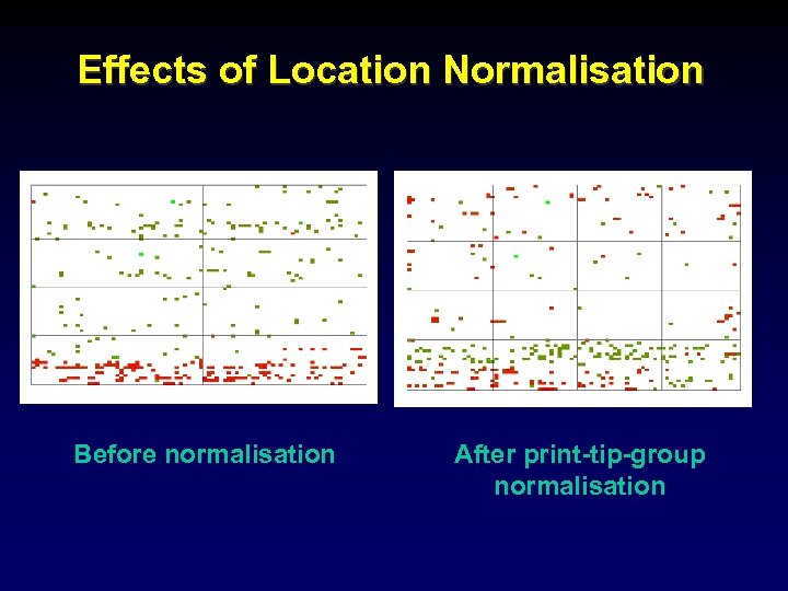Effects of Location Normalisation Before normalisation After print-tip-group normalisation

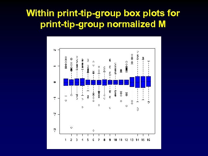Within print-tip-group box plots for print-tip-group normalized M

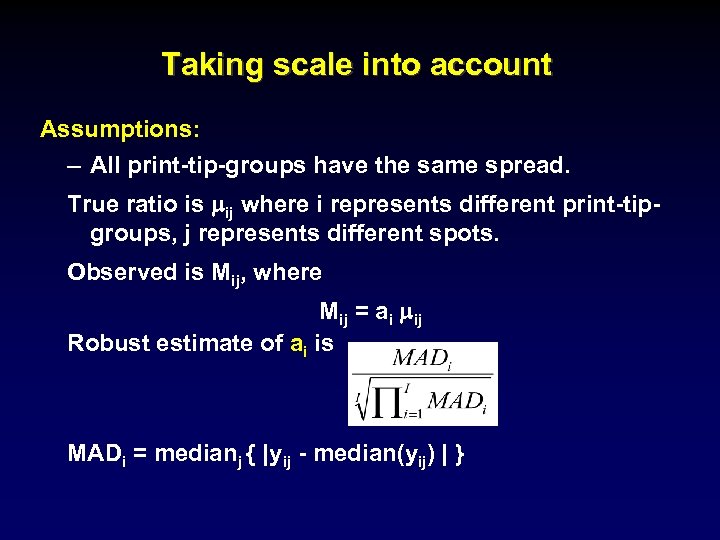Taking scale into account Assumptions: – All print-tip-groups have the same spread. True ratio is mij where i represents different print-tipgroups, j represents different spots. Observed is Mij, where Mij = ai mij Robust estimate of ai is MADi = medianj { |yij - median(yij) | }

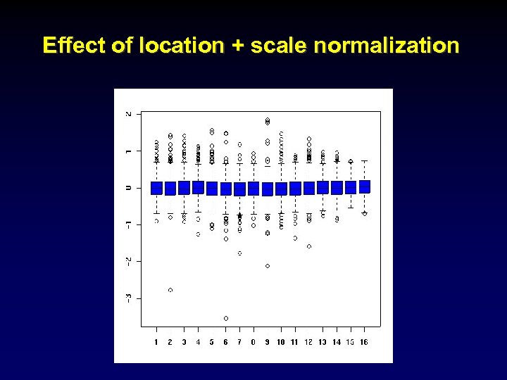Effect of location + scale normalization

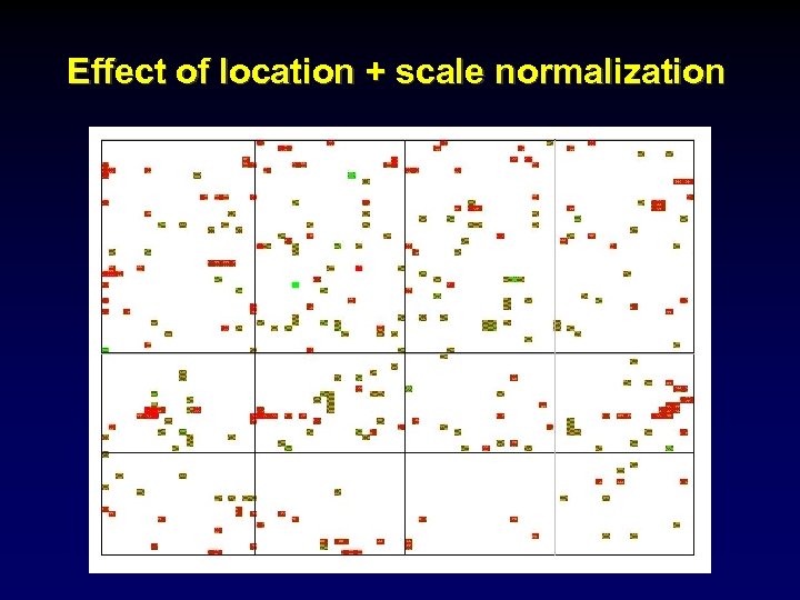Effect of location + scale normalization

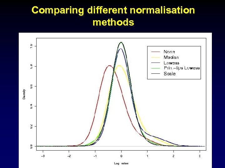Comparing different normalisation methods

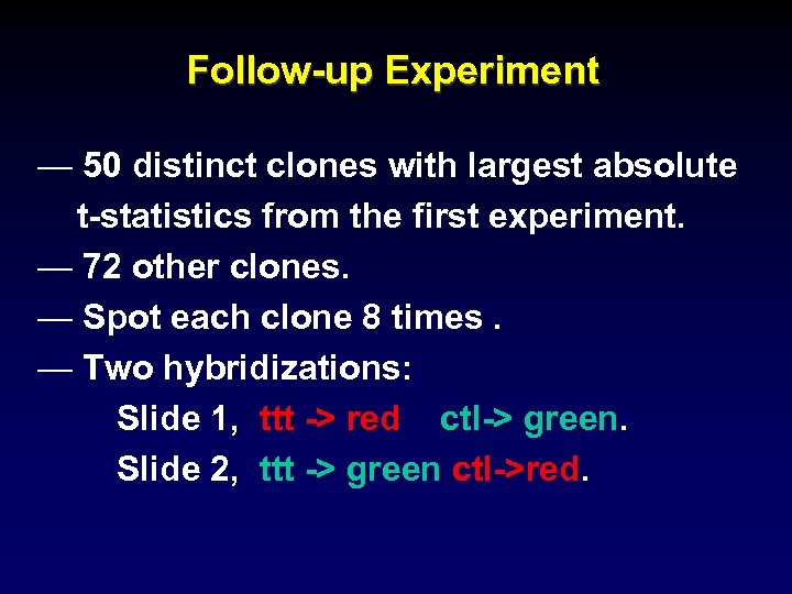Follow-up Experiment — 50 distinct clones with largest absolute t-statistics from the first experiment. — 72 other clones. — Spot each clone 8 times. — Two hybridizations: Slide 1, ttt -> red ctl-> green. Slide 2, ttt -> green ctl->red.

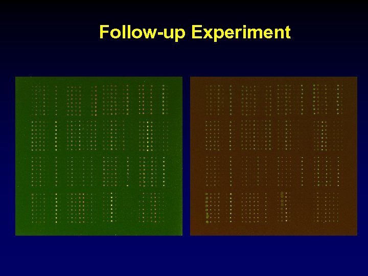Follow-up Experiment

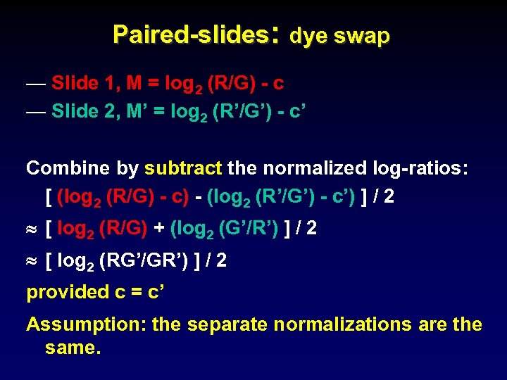Paired-slides: dye swap — Slide 1, M = log 2 (R/G) - c — Slide 2, M’ = log 2 (R’/G’) - c’ Combine by subtract the normalized log-ratios: [ (log 2 (R/G) - c) - (log 2 (R’/G’) - c’) ] / 2 [ log 2 (R/G) + (log 2 (G’/R’) ] / 2 [ log 2 (RG’/GR’) ] / 2 provided c = c’ Assumption: the separate normalizations are the same.

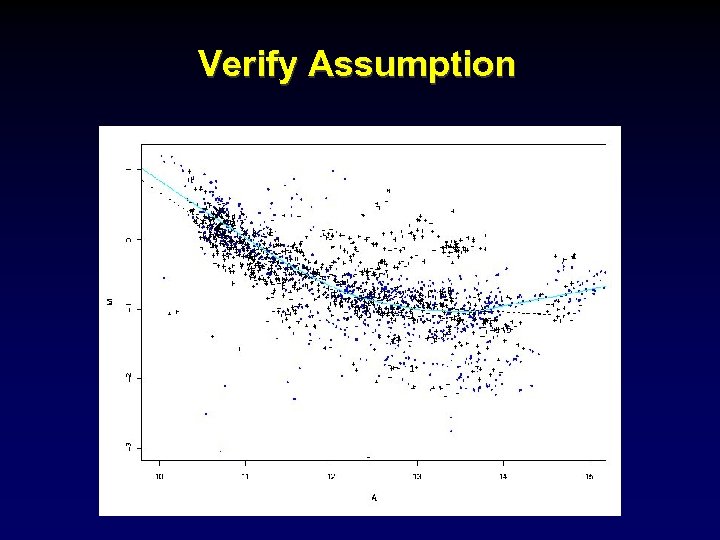Verify Assumption

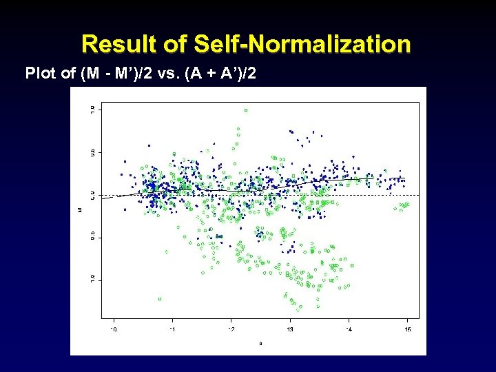Result of Self-Normalization Plot of (M - M’)/2 vs. (A + A’)/2

Summary Case 1: A few genes that are likely to change Within-slide: – Location: print-tip-group lowess normalization. – Scale: for all print-tip-groups, adjust MAD to equal the geometric mean for MAD for all print-tip-groups. Between slides (experiments) : – An extension of within-slide scale normalization (future work). Case 2: Many genes changing (paired-slides) – Self-normalization: taking the difference of the two log-ratios. – Check using controls or known information.

http: //www. stat. berkeley. edu/users/terry/zarray/Html/ Technical Reports from Terry’s group: http: //www. stat. Berkeley. EDU/users/terry/zarray/Html /papersindex. html — Comparison of Discrimination Methods for the Classification of Tumors Using Gene Expression Data — Statistical methods for identifying differentially expressed genes in replicated c. DNA microarray experiments. — Comparison of methods for image analysis on c. DNA microarray data. — Normalization for c. DNA Microarray Data Statistical software R http: //lib. stat. cmu. edu/R/CRAN/

Acknowledgments Terry Speed Sandrine Dudoit Natalie Roberts Ben Bolstad Matt Callow (LBL) John Ngai’s Lab (UCB) Percy Luu Dave Lin Vivian Pang Elva Diaz