9a1c07a4c50eca390a2f60e28eca2cea.ppt
- Количество слайдов: 47
 Non-compartmental analysis and The Mean Residence Time approach A Bousquet-Mélou 1
 Synonymous Mean Residence Time approach Statistical Moment Approach Non-compartmental analysis 2
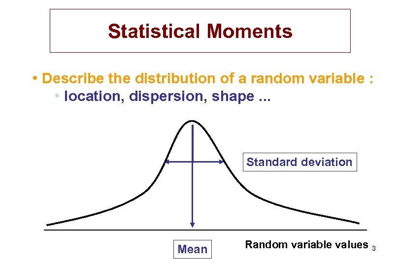 Statistical Moments • Describe the distribution of a random variable : • location, dispersion, shape. . . Standard deviation Mean Random variable values 3
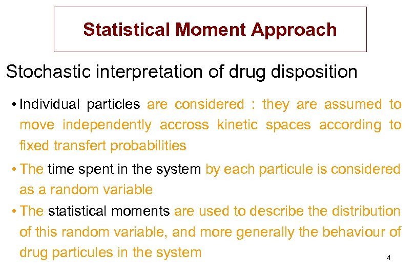 Statistical Moment Approach Stochastic interpretation of drug disposition • Individual particles are considered : they are assumed to move independently accross kinetic spaces according to fixed transfert probabilities • The time spent in the system by each particule is considered as a random variable • The statistical moments are used to describe the distribution of this random variable, and more generally the behaviour of drug particules in the system 4
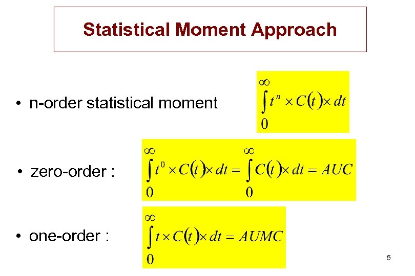 Statistical Moment Approach • n-order statistical moment • zero-order : • one-order : 5
 Statistical Moment Approach Statistical moments in pharmacokinetics. J Pharmacokinet Biopharm. 1978 Dec; 6(6): 547 -58. Yamaoka K, Nakagawa T, Uno T. Statistical moments in pharmacokinetics: models and assumptions. J Pharmacol. 1993 Oct; 45(10): 871 -5. Dunne A. 6
 The Mean Residence Time 7
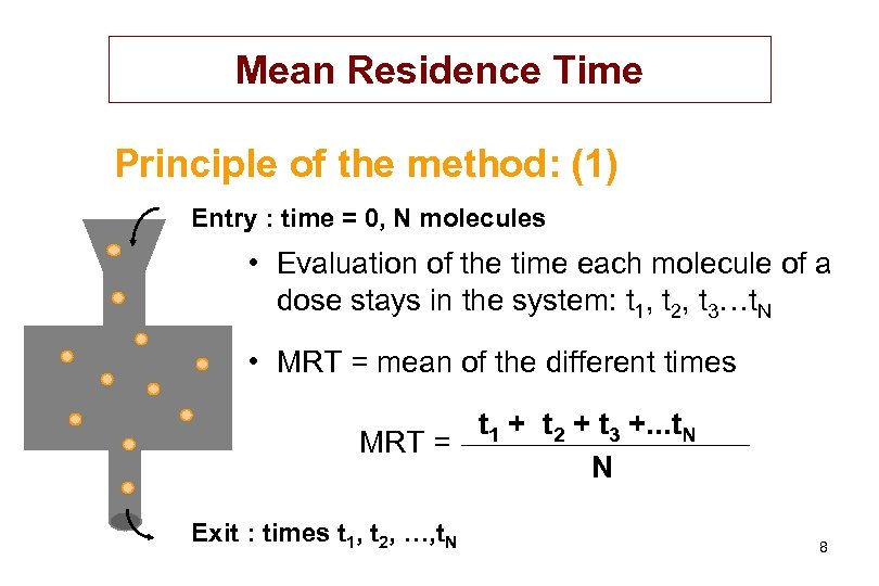 Mean Residence Time Principle of the method: (1) Entry : time = 0, N molecules • Evaluation of the time each molecule of a dose stays in the system: t 1, t 2, t 3…t. N • MRT = mean of the different times t 1 + t 2 + t 3 +. . . t. N MRT = N Exit : times t 1, t 2, …, t. N 8
 Mean Residence Time Principle of the method : (2) • Under minimal assumptions, the plasma concentration curve provides information on the time spent by the drug molecules in the body 9
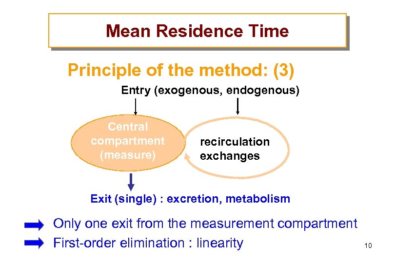 Mean Residence Time Principle of the method: (3) Entry (exogenous, endogenous) Central compartment (measure) recirculation exchanges Exit (single) : excretion, metabolism Only one exit from the measurement compartment First-order elimination : linearity 10
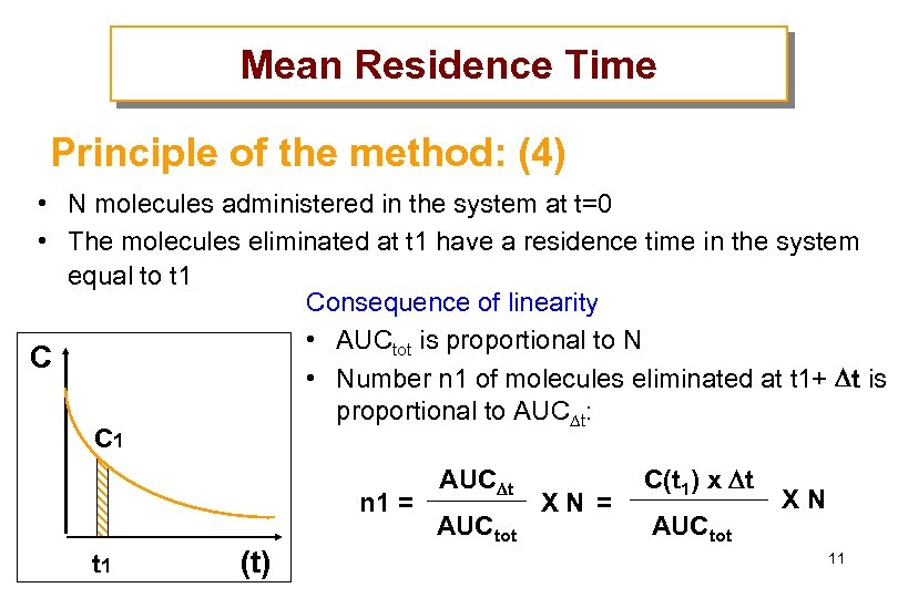 Mean Residence Time Principle of the method: (4) • N molecules administered in the system at t=0 • The molecules eliminated at t 1 have a residence time in the system equal to t 1 Consequence of linearity • AUCtot is proportional to N C • Number n 1 of molecules eliminated at t 1+ t is proportional to AUC t: C 1 n 1 = t 1 (t) AUC t AUCtot XN = C(t 1) x t AUCtot XN 11
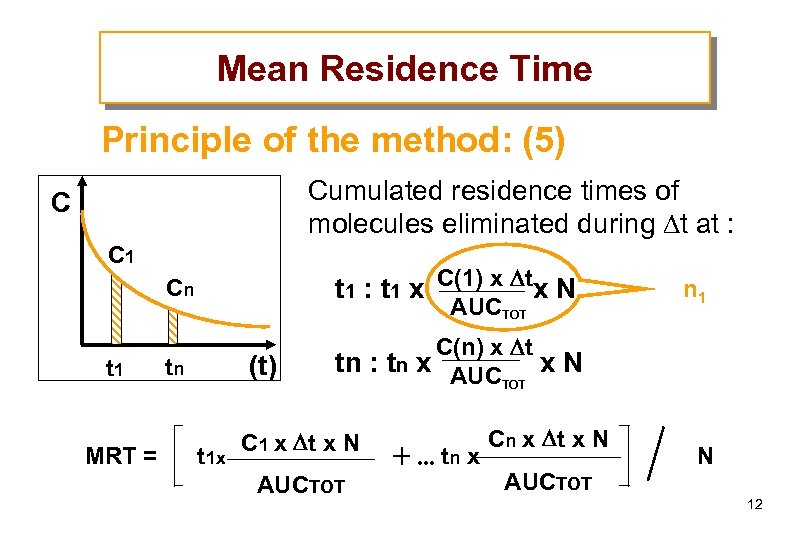 Mean Residence Time Principle of the method: (5) Cumulated residence times of molecules eliminated during t at : C C 1 Cn t 1 MRT = t 1 : t 1 x C(1) x tx N tn C(n) x t tn : tn x AUC x N TOT AUCTOT (t) C 1 x t x N n 1 Cn x t x N t 1 x tn x N AUCTOT 12
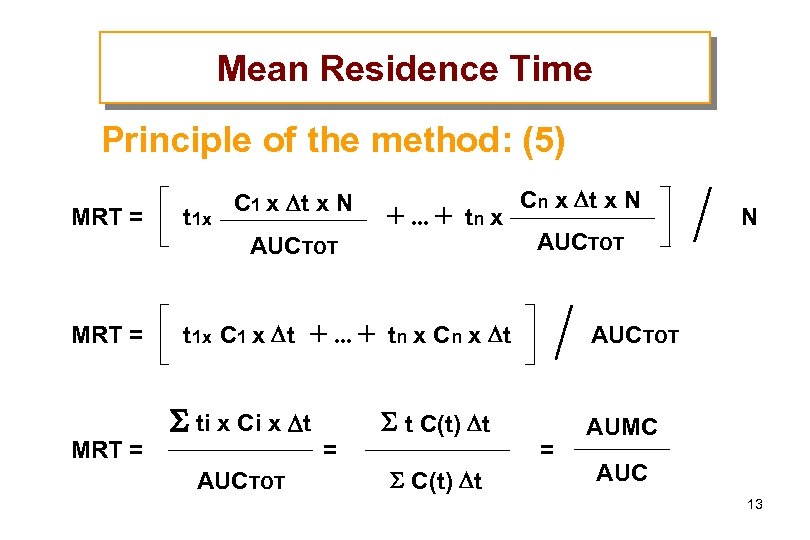 Mean Residence Time Principle of the method: (5) Cn x t x N C 1 x t x N MRT = t 1 x tn x N AUCTOT MRT = t 1 x C 1 x t tn x Cn x t MRT = ti x Ci x t AUCTOT = t C(t) t AUCTOT = AUMC AUC 13
 Mean Residence Time 14
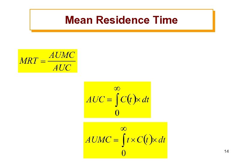
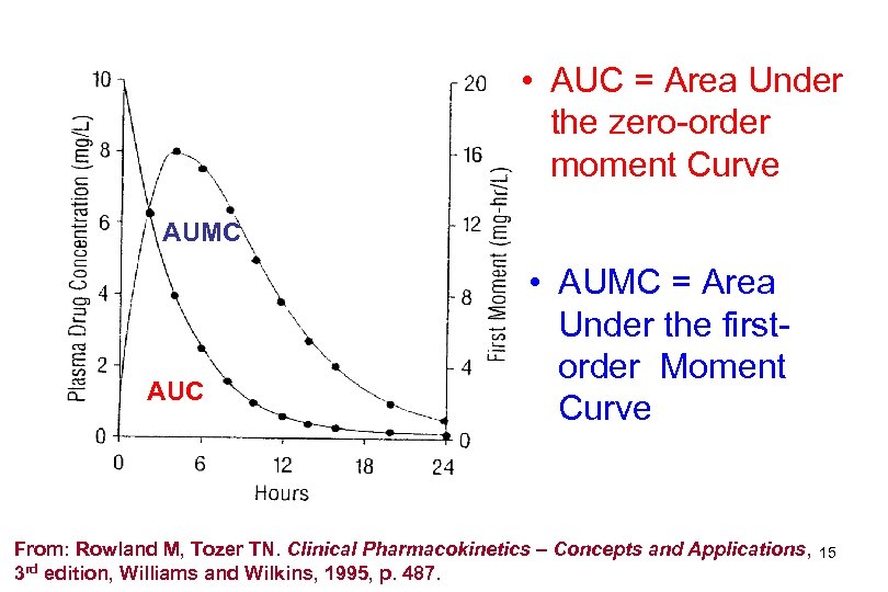 • AUC = Area Under the zero-order moment Curve AUMC AUC • AUMC = Area Under the firstorder Moment Curve From: Rowland M, Tozer TN. Clinical Pharmacokinetics – Concepts and Applications, 3 rd edition, Williams and Wilkins, 1995, p. 487. 15
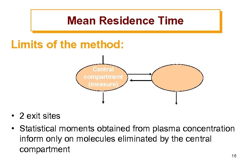 Mean Residence Time Limits of the method: Central compartment (measure) • 2 exit sites • Statistical moments obtained from plasma concentration inform only on molecules eliminated by the central compartment 16
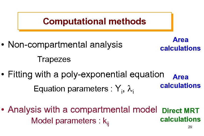
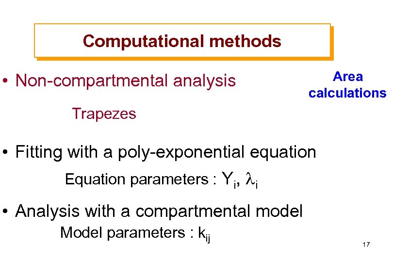 Computational methods • Non-compartmental analysis Area calculations Trapezes • Fitting with a poly-exponential equation Equation parameters : Yi, li • Analysis with a compartmental model Model parameters : kij 17
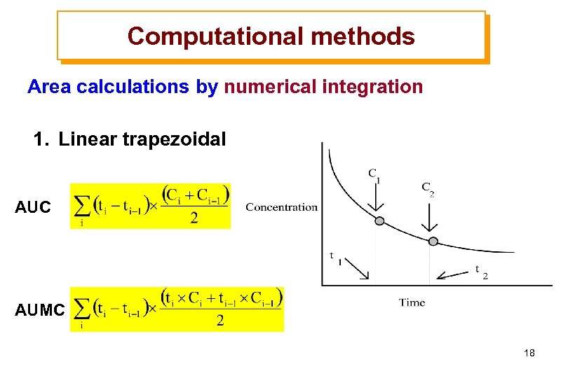 Computational methods Area calculations by numerical integration 1. Linear trapezoidal AUC AUMC 18
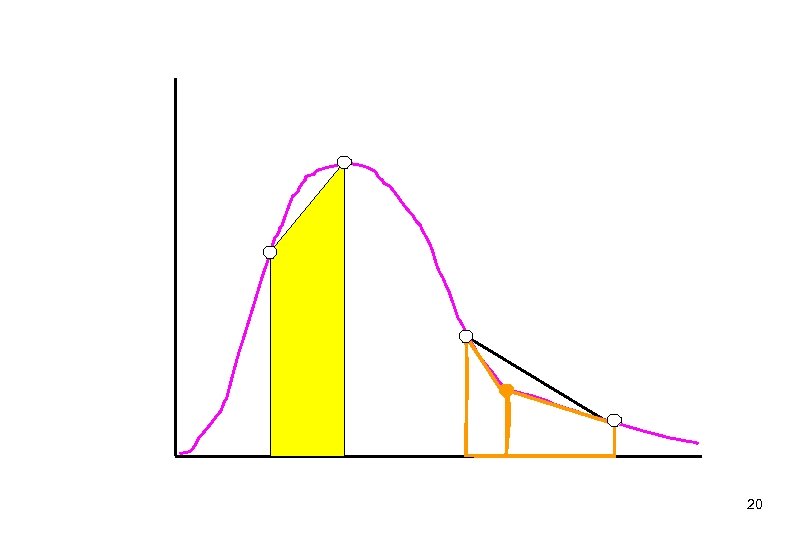
 Computational methods Area calculations by numerical integration 1. Linear trapezoidal Advantages: Simple (can calculate by hand) Disadvantages: • Assumes straight line between data points • If curve is steep, error may be large • Under or over estimation, depending on whether the curve is ascending of descending 19
 20
20
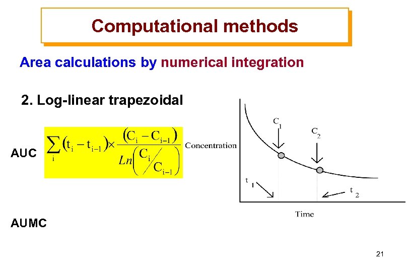 Computational methods Area calculations by numerical integration 2. Log-linear trapezoidal AUC AUMC 21
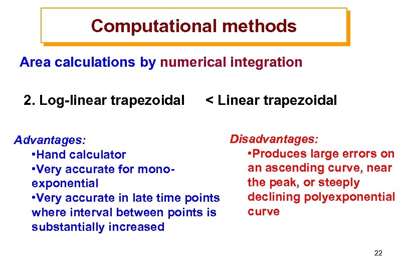 Computational methods Area calculations by numerical integration 2. Log-linear trapezoidal < Linear trapezoidal Disadvantages: Advantages: • Produces large errors on • Hand calculator an ascending curve, near • Very accurate for monothe peak, or steeply exponential declining polyexponential • Very accurate in late time points curve where interval between points is substantially increased 22
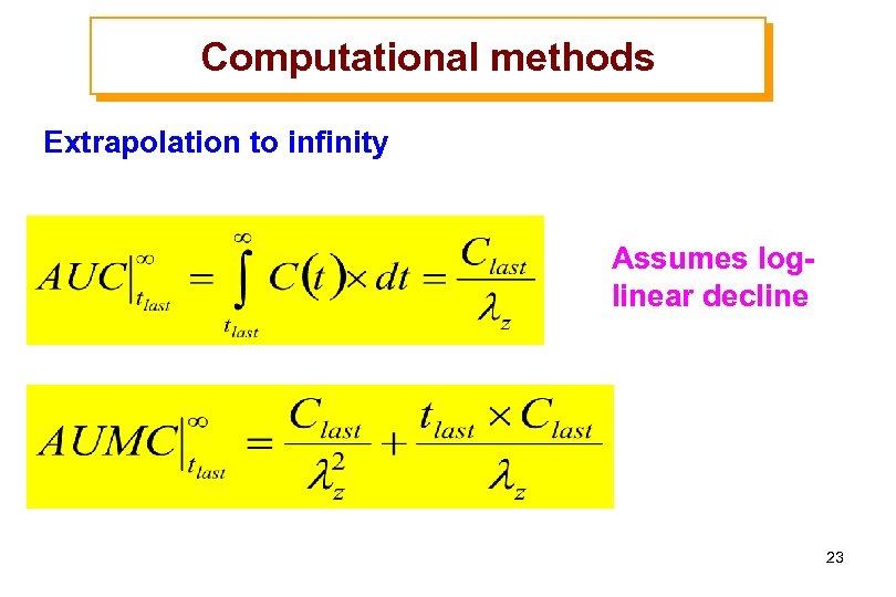 Computational methods Extrapolation to infinity Assumes loglinear decline 23
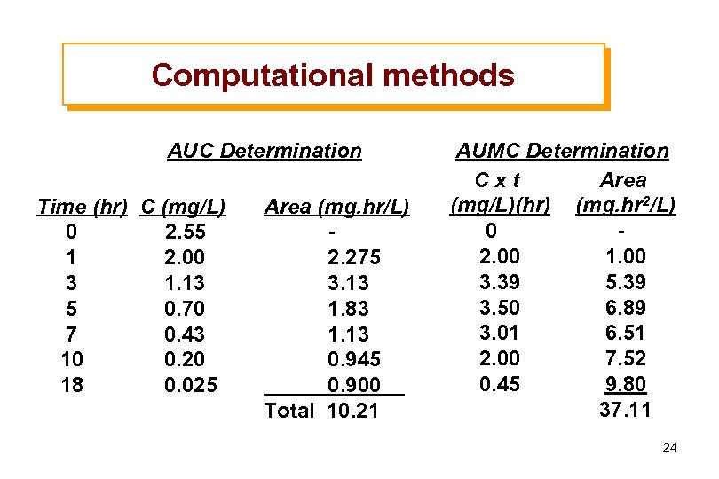 Computational methods AUC Determination Time (hr) C (mg/L) 0 2. 55 1 2. 00 3 1. 13 5 0. 70 7 0. 43 10 0. 20 18 0. 025 Area (mg. hr/L) 2. 275 3. 13 1. 83 1. 13 0. 945 0. 900 Total 10. 21 AUMC Determination Cxt Area (mg/L)(hr) (mg. hr 2/L) 0 2. 00 1. 00 3. 39 5. 39 3. 50 6. 89 3. 01 6. 51 2. 00 7. 52 0. 45 9. 80 37. 11 24
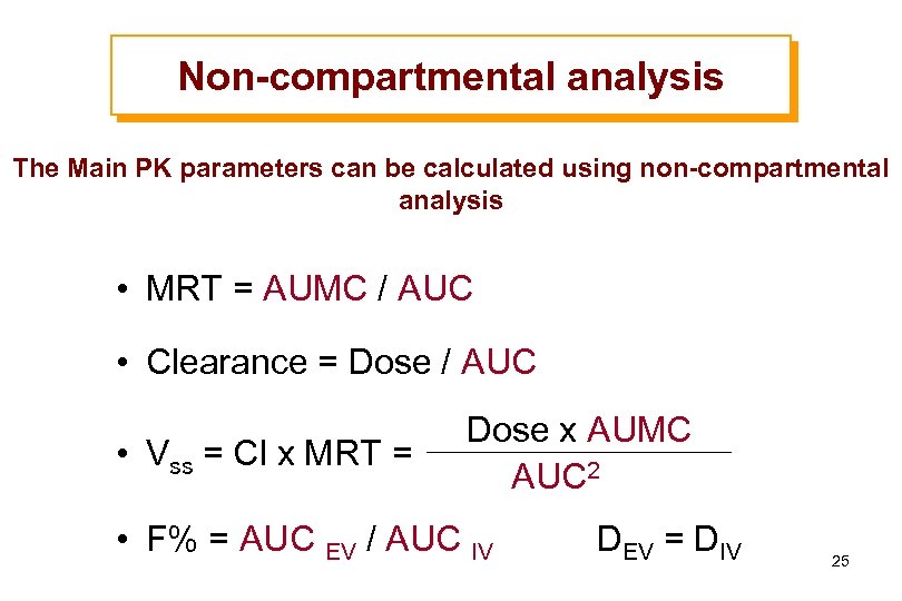 Non-compartmental analysis The Main PK parameters can be calculated using non-compartmental analysis • MRT = AUMC / AUC • Clearance = Dose / AUC • Vss = Cl x MRT = Dose x AUMC AUC 2 • F% = AUC EV / AUC IV DEV = DIV 25
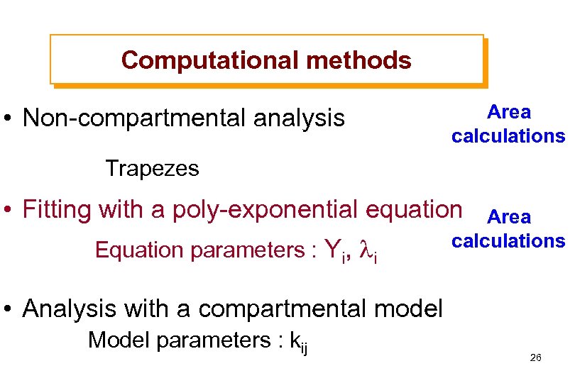 Computational methods • Non-compartmental analysis Area calculations Trapezes • Fitting with a poly-exponential equation Equation parameters : Yi, li Area calculations • Analysis with a compartmental model Model parameters : kij 26
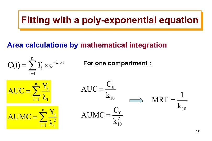 Fitting with a poly-exponential equation Area calculations by mathematical integration For one compartment : 27
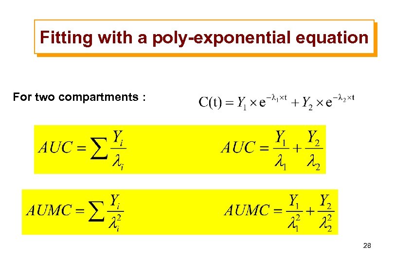 Fitting with a poly-exponential equation For two compartments : 28
 Computational methods • Non-compartmental analysis Area calculations Trapezes • Fitting with a poly-exponential equation Equation parameters : Yi, li • Analysis with a compartmental model Model parameters : kij Area calculations Direct MRT calculations 29
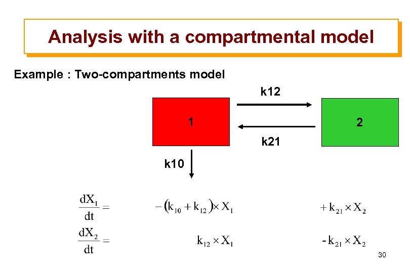 Analysis with a compartmental model Example : Two-compartments model k 12 1 2 k 21 k 10 30
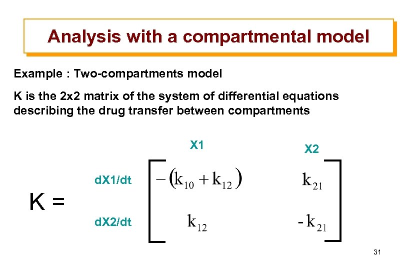 Analysis with a compartmental model Example : Two-compartments model K is the 2 x 2 matrix of the system of differential equations describing the drug transfer between compartments X 1 X 2 d. X 1/dt K= d. X 2/dt 31
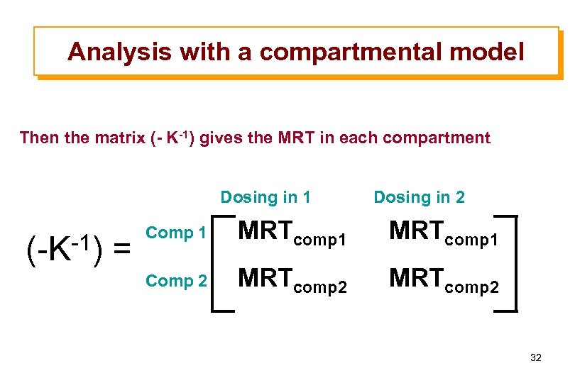 Analysis with a compartmental model Then the matrix (- K-1) gives the MRT in each compartment Dosing in 1 (-K-1) = Dosing in 2 Comp 1 MRTcomp 1 Comp 2 MRTcomp 2 32
 The Mean Residence Times Fundamental property of MRT : ADDITIVITY The mean residence time in the system is the sum of the mean residence times in the compartments of the system • Mean Absorption Time / Mean Dissolution Time • MRT in central and peripheral compartments 33
 The Mean Absorption Time (MAT) 34
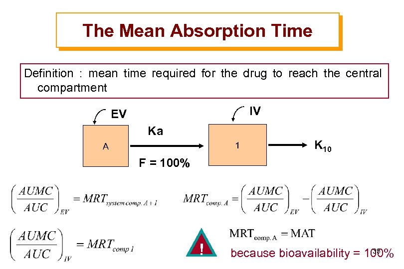 The Mean Absorption Time Definition : mean time required for the drug to reach the central compartment IV EV Ka 1 A K 10 F = 100% ! 35 because bioavailability = 100%
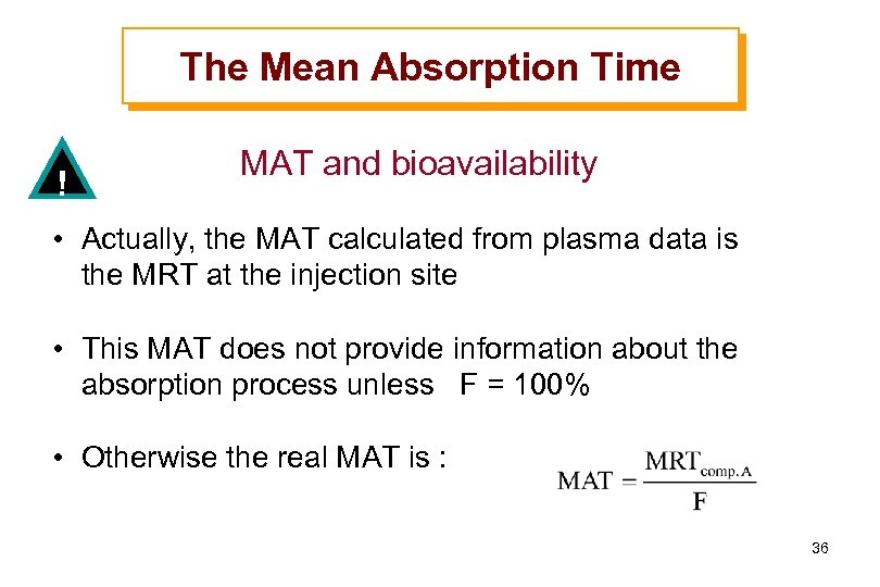 The Mean Absorption Time ! MAT and bioavailability • Actually, the MAT calculated from plasma data is the MRT at the injection site • This MAT does not provide information about the absorption process unless F = 100% • Otherwise the real MAT is : 36
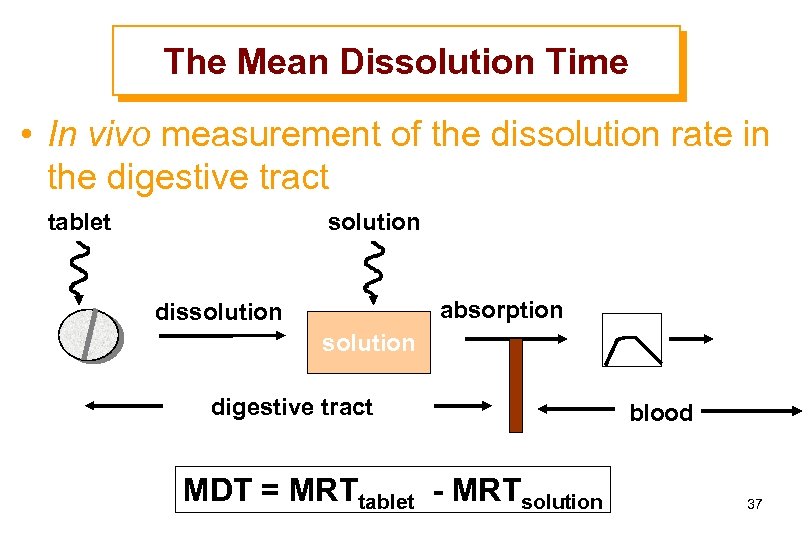 The Mean Dissolution Time • In vivo measurement of the dissolution rate in the digestive tract tablet solution absorption dissolution digestive tract MDT = MRTtablet - MRTsolution blood 37
 Mean Residence Time in the Central Compartment (MRTC) and in the Peripheral (Tissues) Compartment (MRTT) 38
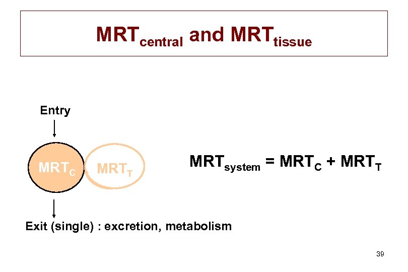 MRTcentral and MRTtissue Entry MRTC MRTT MRTsystem = MRTC + MRTT Exit (single) : excretion, metabolism 39
 The Mean Transit Time (MTT) 40
 The Mean Transit Times (MTT) • Definition : – Average interval of time spent by a drug particle from its entry into the compartment to its next exit – Average duration of one visit in the compartment • Computation : – The MTT in the central compartment can be calculated for plasma concentrations after i. v. 41
 The Mean Residence Number (MRN) 42
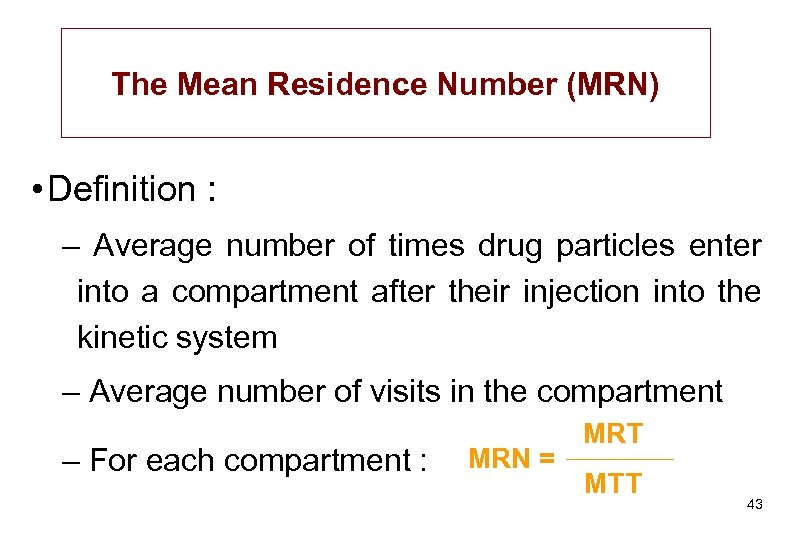 The Mean Residence Number (MRN) • Definition : – Average number of times drug particles enter into a compartment after their injection into the kinetic system – Average number of visits in the compartment – For each compartment : MRN = MRT MTT 43
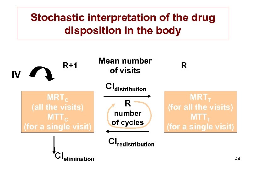 Stochastic interpretation of the drug disposition in the body IV R+1 MRTC (all the visits) MTTC (for a single visit) Mean number of visits Cldistribution R number of cycles R MRTT (for all the visits) MTTT (for a single visit) Clredistribution Clelimination 44
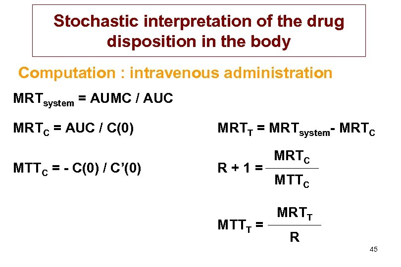 Stochastic interpretation of the drug disposition in the body Computation : intravenous administration MRTsystem = AUMC / AUC MRTC = AUC / C(0) MTTC = - C(0) / C’(0) MRTT = MRTsystem- MRTC R+1= MTTT = MRTC MTTC MRTT R 45
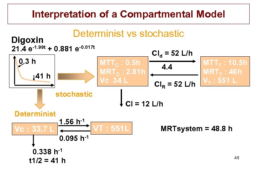 Interpretation of a Compartmental Model Determinist vs stochastic Digoxin 21. 4 e-1. 99 t + 0. 881 e-0. 017 t 0. 3 h MTTC : 0. 5 h MRTC : 2. 81 h Vc 34 L 41 h Cld = 52 L/h MTTT : 10. 5 h 4. 4 MRTT : 46 h Cl. R = 52 L/h VT : 551 L stochastic Cl = 12 L/h Determinist Vc : 33. 7 L 1. 56 h-1 VT : 551 L MRTsystem = 48. 8 h 0. 095 h-1 0. 338 h-1 t 1/2 = 41 h 46
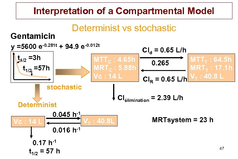 Interpretation of a Compartmental Model Gentamicin Determinist vs stochastic y =5600 e-0. 281 t + 94. 9 e-0. 012 t t 1/2 =3 h t 1/2 =57 h stochastic MTTC : 4. 65 h MTTT : 64. 5 h 0. 265 MRTC : 5. 88 h MRTT : 17. 1 h Vc : 14 L Cl. R = 0. 65 L/h VT : 40. 8 L Determinist 0. 045 h-1 VT : 40. 8 L Vc : 14 L 0. 016 h-1 0. 17 h-1 t 1/2 = 57 h Cld = 0. 65 L/h Clélimination = 2. 39 L/h MRTsystem = 23 h 47


