6c104bb9afc466a01592cf30b72ffec3.ppt
- Количество слайдов: 46
 No 08. Chapter 9 The IS-LM/AD-AS Model: A General Framework for Macroeconomic Analysis
 Chapter 9. Introduction l l This chapter integrates the elements of our model that were separately presented in chapters 3, 4, and 7, covering labor, goods, and asset markets. It develops a graphical depiction of our theory that is called the IS-LM/AD-AS model. l l IS and LM refer to two equilibrium conditions in the model (investment equals saving; money demand, or liquidity preference, equals money supply). AD and AS refer to aggregate demand aggregate supply.
 The FE Line l l I will be using some diagrams that plot the real rate of interest, r, and output Y on the axes. Recall that labor market equilibrium determines a quantity of labor, which, via the production function, determines a full-employment level of output. l Since that level of output presumably does not depend on the rate of interest, we can plot the full-employment line as a vertical line in a diagram in which r and Y appear on vertical and horizontal axes.
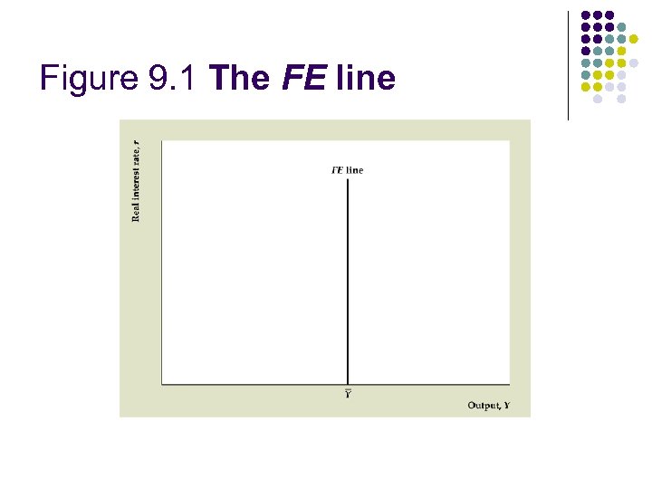 Figure 9. 1 The FE line
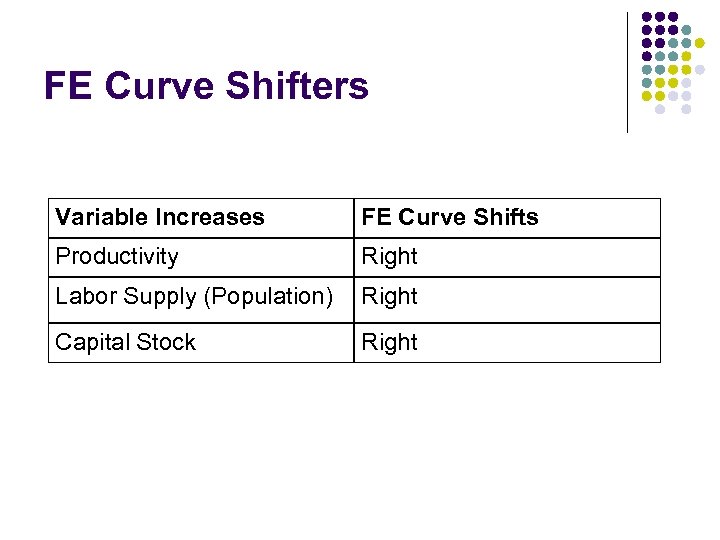 FE Curve Shifters Variable Increases FE Curve Shifts Productivity Right Labor Supply (Population) Right Capital Stock Right
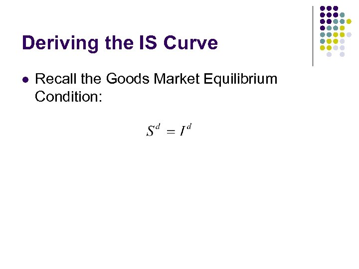 Deriving the IS Curve l Recall the Goods Market Equilibrium Condition:
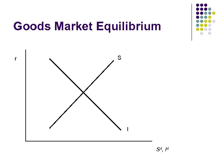 Goods Market Equilibrium r S I Sd, I d
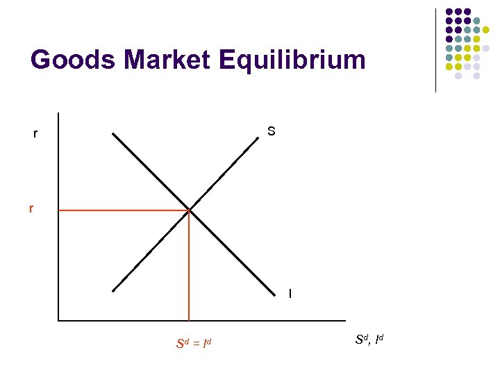 Goods Market Equilibrium S r r I Sd = I d Sd, I d
 Consider a Rise in Income l As income rises, the desired saving curve shifts right, and the equilibrium rate of interest falls as we slide down the desired investment curve (next slide).
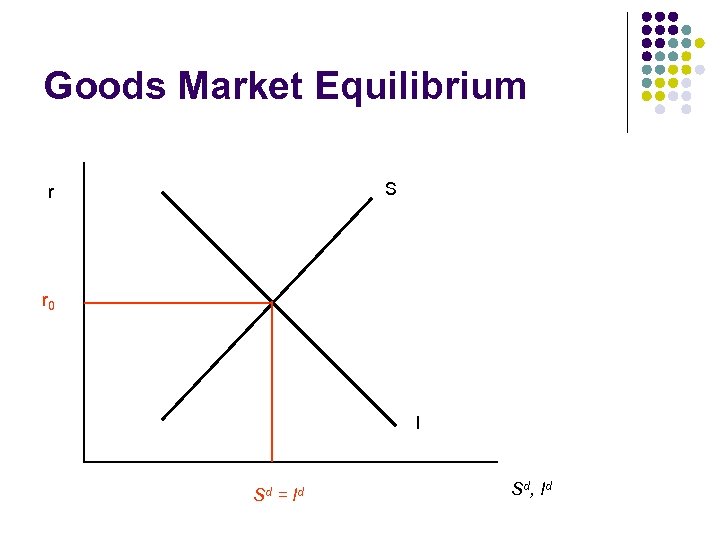 Goods Market Equilibrium S r r 0 I Sd = I d Sd, I d
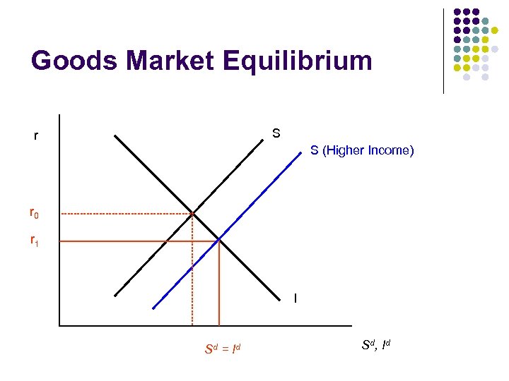 Goods Market Equilibrium S r S (Higher Income) r 0 r 1 I Sd = I d Sd, I d
 Deriving IS l l The previous slide shows that as income varies and goods market equilibrium is maintained, a higher value of income is associated with a lower value of the expected real interest rate Plot the income-interest rate pairs that satisfy the goods market equilibrium condition to get the IS curve l The inverse relationship between income and interest rate implies that the IS curve is downward sloping
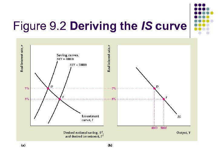 Figure 9. 2 Deriving the IS curve
 Shifting IS l l Recall that IS was derived by considering how the desired saving curve moved along the desired investment curve as income changed. Suppose a shock (say a government spending increase) causes saving to decline at each level of income l l l Then the interest rate is higher at each level of income. Then we must redraw IS, with higher r for each level of Y. IS has shifted to the right. For other shocks that shift saving or investment schedules, we can also infer how IS shifts.
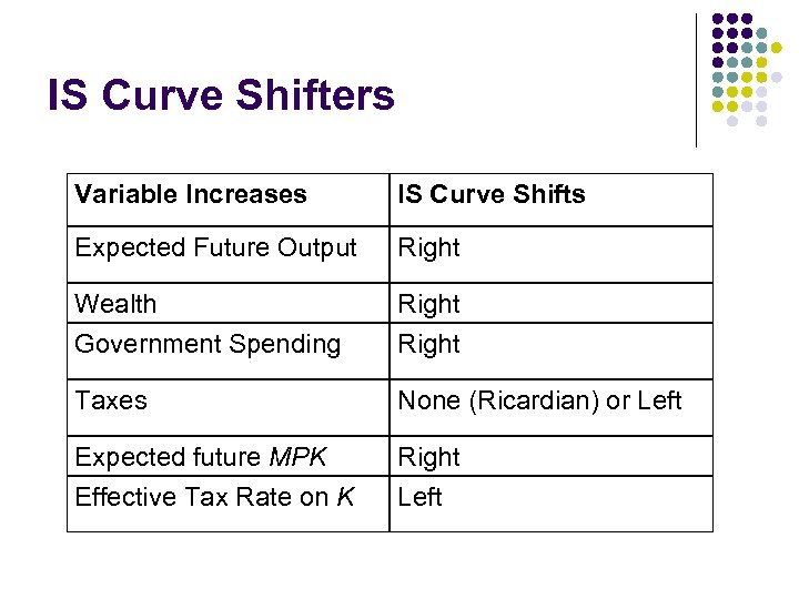 IS Curve Shifters Variable Increases IS Curve Shifts Expected Future Output Right Wealth Right Government Spending Right Taxes None (Ricardian) or Left Expected future MPK Effective Tax Rate on K Right Left
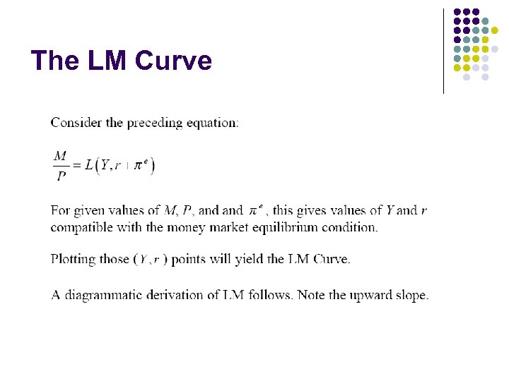
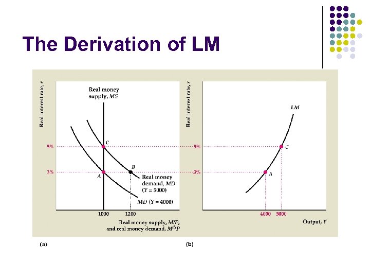
 The LM Curve l l The IS plots income interest-rate pairs such that desired spending is equal to output, or desired saving is equal to desired investment We will now derive the LM curve, which plots income-interest rate pairs such that the quantity of money demanded is equal to the quantity of money supplied.
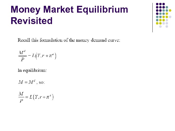 Money Market Equilibrium Revisited
 The LM Curve
 The Derivation of LM
 LM Curve Shifters Variable Increases Nominal Money Supply Price Level Expected Inflation LM Curve Shifts Right Left Right Nominal interest rate on Left money im Anything Else Left Increasing the Demand for Money
 General Equilibrium in the ISLM Model l In general equilibrium, all markets satisfy their respective equilibrium conditions. l l Labor, Goods, and Money Markets Must all be in equilibrium. The logic of general equilibrium: l l l The labor market determines output. Given output (income) the goods market then determines an interest rate. Given output, the interest rate, and the expected inflation rate, then the money market determines the price level.
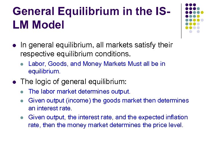
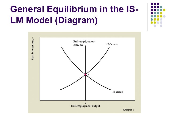 General Equilibrium in the ISLM Model (Diagram)
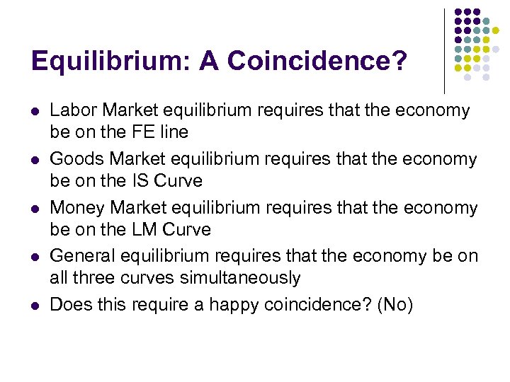 Equilibrium: A Coincidence? l l l Labor Market equilibrium requires that the economy be on the FE line Goods Market equilibrium requires that the economy be on the IS Curve Money Market equilibrium requires that the economy be on the LM Curve General equilibrium requires that the economy be on all three curves simultaneously Does this require a happy coincidence? (No)
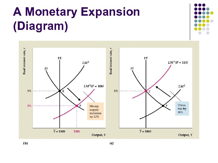
 Consider a Monetary Expansion l l l Suppose that the money supply increases. This shifts the LM Curve to the right. Normally, an increase in the money supply, holding other things equal, would put downward pressure on the rate of interest l People are willing to hold the greater supply of money if the interest rate is lower as the economy slides down the IS curve. But at the IS-LM intersection, desired spending is greater than the full employment level of output. The excess of spending over output produced puts upward pressure on the price level, returning LM to its original position, and the economy to its original equilibrium
 A Monetary Expansion (Diagram)
 Review on Equilibrium To review, output is determined by the FE line l Given output the intersection of IS and FE determines the interest rate l Finally, the price level adjusts so that LM intersects both IS and FE l
 A Digression on Goods Market Equilibrium l l l Our goods market equilibrium condition requires that desired spending be equal to output produced However, this is not really a typical demand-supply equilibrium notion The goods market equilibrium condition may be better thought of as a demand consistency condition: l l That is, if a certain output is produced it generates income, and that income generates spending. If the spending generated is just sufficient to buy up the output produced, then the demand consistency condition is satisfied. We need the FE line, reflecting limitations imposed by resource availability and technology, to put a supply-side constraint on our theory
 Timing of Movement to Equilibrium l l Our model, as formulated, does not tell us the order in which variables move—we just infer that the economy moves from one equilibrium to another (after a shock). Here are some thoughts on timing: l l Interest rates (and financial markets generally) adjust very quickly Nominal (and real) wages adjust slowly (often wages are set for long periods of time Prices may also adjust slowly The goods market adjusts with intermediate speed (we often see unanticipated inventory movements, but firms may alter production before revising prices)
 Timing of Movement to Equilibrium (More) l l l When the money supply increases, the interest rate falls (the Fed buys bonds, driving up the price, and lowering the rate of interest). Desired spending increases, so firms see inventories declining. Firms increase production (and workers work more). Firms initially respond by producing more, but will eventually adjust prices upward; workers will also negotiate higher nominal wages. When prices rise, the real money supply falls, LM shifts back to the left, and the interest rate, the rate of output, and the real wage all return to original levels
 A Look Ahead: Keynesian and Classical Views l l l We will say much more about “Keynesian” and “Classical” macroeconomic theories Keynesians emphasize the short-term rigidity of prices and wages Classical economists emphasize that all markets reach equilibria rather quickly
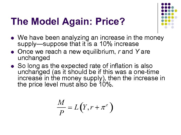 The Model Again: Price? l l l We have been analyzing an increase in the money supply—suppose that it is a 10% increase Once we reach a new equilibrium, r and Y are unchanged So long as the expected rate of inflation is also unchanged (as it should be if this was a one-time increase in the money supply), then the increase in the price level must also be 10%.
 What Happened to Wages? l The price level rose 10%, but the real wage is unchanged l l Labor demand supply curves never moved, so the equilibrium real wage has not changed either But if the real wage is unchanged, and the price level has increased by 10%, then the nominal wage must also increase by 10%
 Money Neutrality l l l In our thought experiment, an increase in the money supply affected nominal variables (P and W) but not real variables (Y, C, I, r, W/P) “Money Neutrality” is the proposition that an increase in the money supply has no real effects Money neutrality holds (almost) immediately in the Classical view, but only after a considerable lag in the Keynesian view
 Steady Money Growth l l We just considered a one-time increase in M, which eventually was followed by an equiproportional increase in P Suppose that money is increasing steadily, not just once l l For example, money and prices might each be growing steadily at a 4% rate In such a situation, LM is not moving at all, and output and the real rate of interest will be constant.
 Aggregate Demand Aggregate Supply l l l We have now specified a complete model However, sometimes it is convenient to look at the model differently—with a different diagram We next introduce AD and AS curves l l These curves plot output, Y, and the price level, P. These diagrams allow us to focus attention on the determination of the price level, which was not directly visible in the IS-LM diagram.
 The AD Curve l l Consider the IS-LM diagram. A given LM curve is drawn for a fixed level of P. If P changes, then the LM curve shifts. Consider various levels of P. l l l For each price level, draw the appropriate LM curve The sequence of IS-LM intersections determines Y values to be associated with each level of P. Plotting these P-Y pairs yields the aggregate demand (AD) curve.
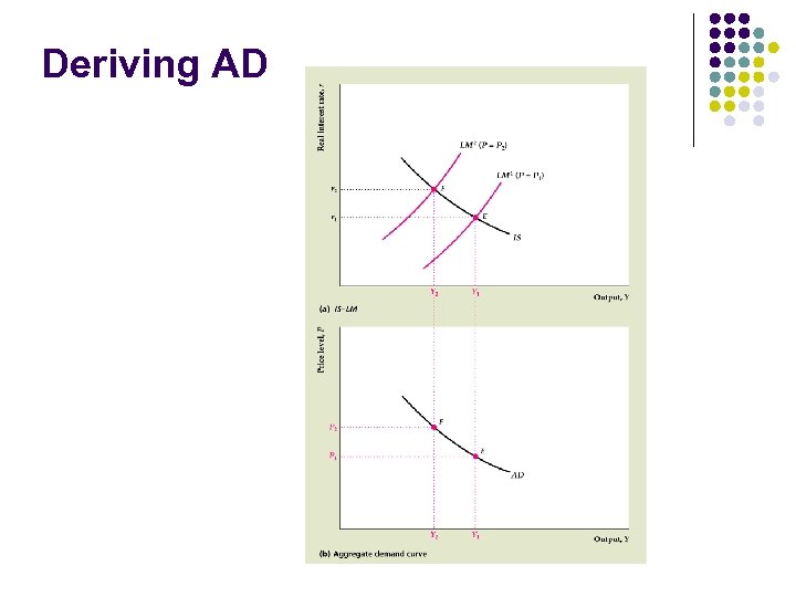 Deriving AD
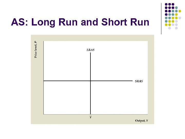
 The Long Run Aggregate Supply Curve l When all markets clear, we are in long-run equilibrium. l l Note: This is not necessarily a matter of time. In the classical model, when all markets equilibrate instantaneously, then we reach the long-run immediately. The AS curve plots output supplied versus the price level. Output supplied is determined by the labor market and the production function; it is the full employment level of output, . Output supplied does not vary with P, so the AS curve is vertical at.
 Aggregate Supply in the Short. Run l l l Assume that the short-run is a time frame in which the price level is fixed, and the quantity of output is determined by demand (whatever that level may be) So the AS curve is horizontal at a given price level Our original labor market equilibrium model has been discarded for the short run l The short-run horizontal AS curve is really only a feature of Keynesian interpretations of our theory
 AS: Long Run and Short Run
 Long-run and Short-run Equilibria l l l In long-run equilibrium, the economy must be on AD, SRAS, and LRAS. In a short-run equilibrium, the economy must be on AD and SRAS. To go to a new long-run equilibrium, price (and SRAS) must shift. Note that our assumptions now make it clear that an increase in AD can lead to an increase in output in the short-run, but an increase in price in the long-run The vertical long-run supply illustrates the money neutrality property l Increases in M, causing increases in AD, do not change output, but they do change P.
 AD Shifters l l Any variable that shifts IS or LM, with the exception of P, will also shift AD The direction of the shift is determined by whether the IS-LM diagram shows an increase in income as a result of the shift in the IS-LM diagram: if IS and LM intersect at a higher level of income, then the AD curve shifts to the right. l At any price level, if IS and AD determine a higher level of income, then that price level is now associated with a higher level on income on AD.
 LRAS Shifters l l The LRAS curve will change when the full employment level of output changes This means that it is shifted by the same variables that shift the FE Curve: l l l Productivity Labor supply Capital stock
 SRAS Shifters l The SRAS curve shifts only when the price level changes from one “fixed” level to another l This period price might be fixed at a given level, but in a future period it might be fixed at some other level
 Upcoming Chapters l In the next two chapters, we will use the ISLM / AS-AD model to illustrate short- and long-run consequences of a variety of shocks to the economy
 The End


