NIFS Data Reduction Richard Mc Dermid Gemini Data

NIFS Data Reduction Richard Mc. Dermid Gemini Data Reduction Workshop Tucson, July 2010

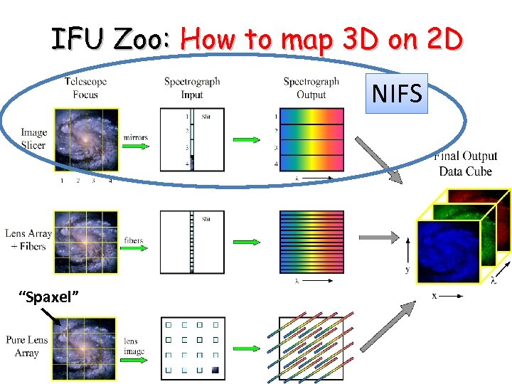IFU Zoo: How to map 3 D on 2 D NIFS “Spaxel”

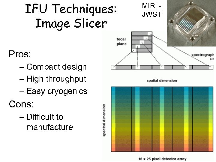IFU Techniques: Image Slicer Pros: – Compact design – High throughput – Easy cryogenics Cons: – Difficult to manufacture MIRI JWST

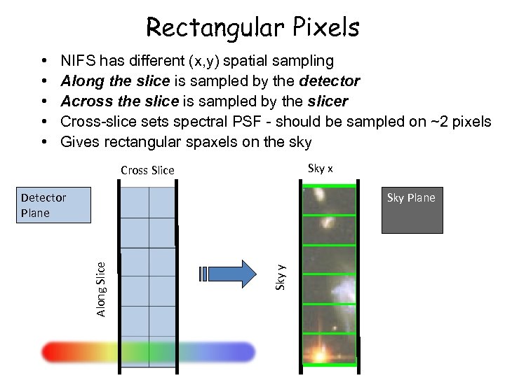Rectangular Pixels • • • NIFS has different (x, y) spatial sampling Along the slice is sampled by the detector Across the slice is sampled by the slicer Cross-slice sets spectral PSF - should be sampled on ~2 pixels Gives rectangular spaxels on the sky Sky x Cross Slice Sky Plane Sky y Along Slice Detector Plane

NIFS • • Near-infrared Integral Field Spectrograph Cryogenic slicer design Z, J, H, K bands, R~5, 000 One spatial setting: – 3”x 3” Fo. V – 0. 1”x 0. 04” sampling • Optimized for use with AO • Science: young stars, exo-planets, solar system, black holes, jets, stellar populations, hi-z galaxies….

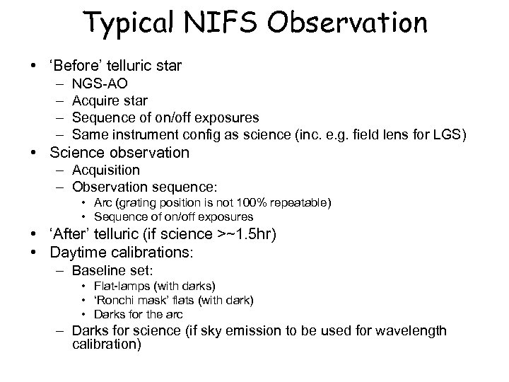Typical NIFS Observation • ‘Before’ telluric star – – NGS-AO Acquire star Sequence of on/off exposures Same instrument config as science (inc. e. g. field lens for LGS) • Science observation – Acquisition – Observation sequence: • Arc (grating position is not 100% repeatable) • Sequence of on/off exposures • ‘After’ telluric (if science >~1. 5 hr) • Daytime calibrations: – Baseline set: • Flat-lamps (with darks) • ‘Ronchi mask’ flats (with dark) • Darks for the arc – Darks for science (if sky emission to be used for wavelength calibration)

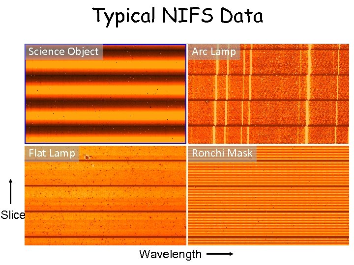Typical NIFS Data Science Object Arc Lamp Flat Lamp Ronchi Mask Slice Wavelength

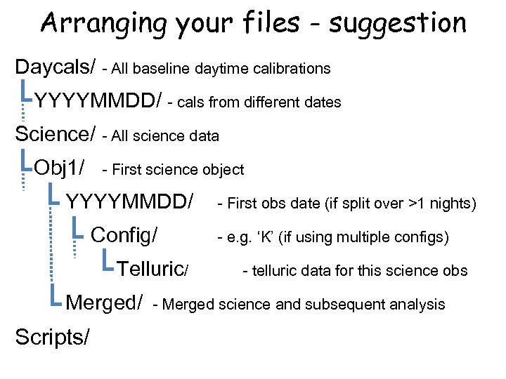Arranging your files - suggestion Daycals/ - All baseline daytime calibrations YYYYMMDD/ - cals from different dates Science/ - All science data Obj 1/ - First science object YYYYMMDD/ Config/ Telluric/ Merged/ Scripts/ - First obs date (if split over >1 nights) - e. g. ‘K’ (if using multiple configs) - telluric data for this science obs - Merged science and subsequent analysis

NIFS Reduction: Example scripts • Three IRAF scripts on the web: – Calibrations – Telluric – Science • Form the basis of this tutorial • Data set: – Science object (star) – Telluric correction star – Daytime calibrations • Update the path and file numbers at the top of each script • Excellent starting point for basic reduction

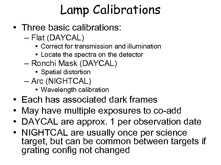Lamp Calibrations • Three basic calibrations: – Flat (DAYCAL) • Correct for transmission and illumination • Locate the spectra on the detector – Ronchi Mask (DAYCAL) • Spatial distortion – Arc (NIGHTCAL) • Wavelength calibration • • Each has associated dark frames May have multiple exposures to co-add DAYCAL are approx. 1 per observation date NIGHTCAL are usually once per science target, but can be common between targets if grating config not changed

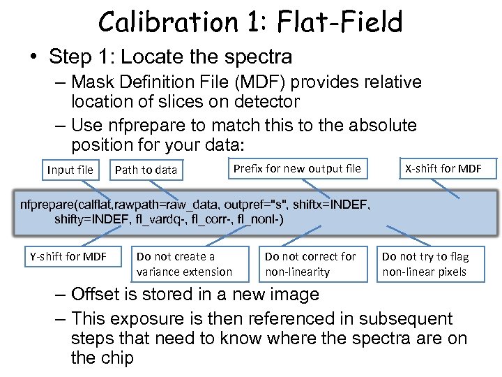Calibration 1: Flat-Field • Step 1: Locate the spectra – Mask Definition File (MDF) provides relative location of slices on detector – Use nfprepare to match this to the absolute position for your data: Input file Path to data Prefix for new output file X-shift for MDF nfprepare(calflat, rawpath=raw_data, outpref="s", shiftx=INDEF, shifty=INDEF, fl_vardq-, fl_corr-, fl_nonl-) Y-shift for MDF Do not create a variance extension Do not correct for non-linearity Do not try to flag non-linear pixels – Offset is stored in a new image – This exposure is then referenced in subsequent steps that need to know where the spectra are on the chip

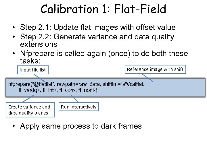Calibration 1: Flat-Field • Step 2. 1: Update flat images with offset value • Step 2. 2: Generate variance and data quality extensions • Nfprepare is called again (once) to do both these tasks: Reference image with shift Input file list nfprepare("@flatlist”, rawpath=raw_data, shiftim="s"//calflat, fl_vardq+, fl_int+, fl_corr-, fl_nonl-) Create variance and data quality planes Run interactively • Apply same process to dark frames

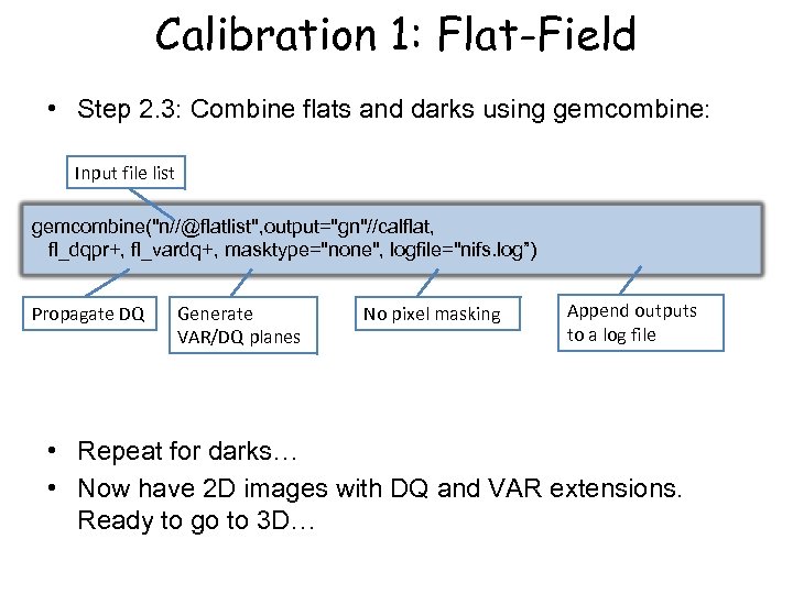Calibration 1: Flat-Field • Step 2. 3: Combine flats and darks using gemcombine: Input file list gemcombine("n//@flatlist", output="gn"//calflat, fl_dqpr+, fl_vardq+, masktype="none", logfile="nifs. log”) Propagate DQ Generate VAR/DQ planes No pixel masking Append outputs to a log file • Repeat for darks… • Now have 2 D images with DQ and VAR extensions. Ready to go to 3 D…

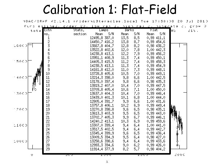
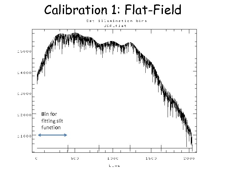
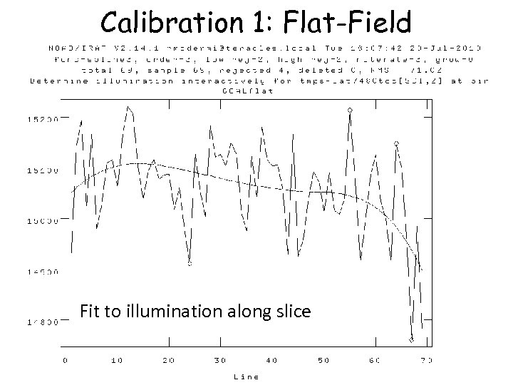
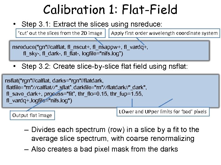Calibration 1: Flat-Field • Step 3. 1: Extract the slices using nsreduce: ‘cut’ out the slices from the 2 D image Apply first order wavelength coordinate system nsreduce("gn"//calflat, fl_nscut+, fl_nsappw+, fl_vardq+, fl_sky-, fl_dark-, fl_flat-, logfile="nifs. log”) • Step 3. 2: Create slice-by-slice flat field using nsflat: nsflat("rgn"//calflat, darks="rgn"//flatdark, flatfile="rn"//calflat//"_sflat”, darkfile="rn"//flatdark//"_dark", fl_save_dark+, process="fit”, thr_flo=0. 15, thr_fup=1. 55, fl_vardq+, logfile="nifs. log") Output flat image LOwer and UPper limits for ‘bad’ pixels – Divides each spectrum (row) in a slice by a fit to the average slice spectrum, with coarse renormalizing – Also creates a bad pixel mask from the darks

Calibration 1: Flat-Field

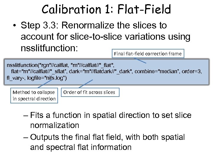Calibration 1: Flat-Field • Step 3. 3: Renormalize the slices to account for slice-to-slice variations using nsslitfunction: Final flat-field correction frame nsslitfunction("rgn"//calflat, "rn"//calflat//"_flat", flat="rn"//calflat//"_sflat”, dark="rn"//flatdark//"_dark", combine="median”, order=3, fl_vary-, logfile="nifs. log”) Method to collapse in spectral direction Order of fit across slices – Fits a function in spatial direction to set slice normalization – Outputs the final flat field, with both spatial and spectral flat information

Calibration 1: Flat-Field Bin for fitting slit function

Calibration 1: Flat-Field Fit to illumination along slice

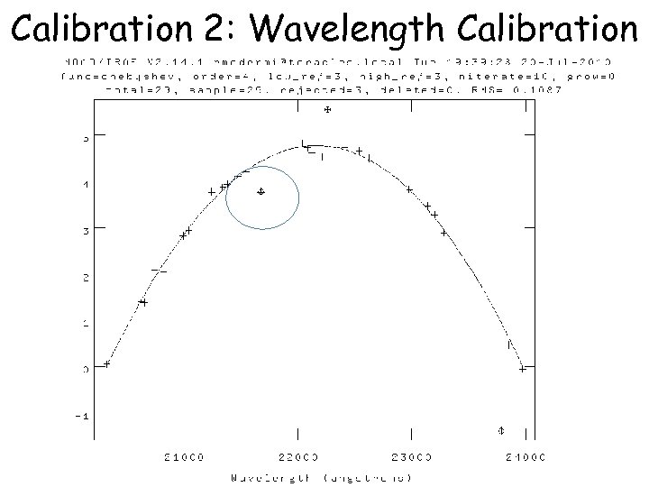
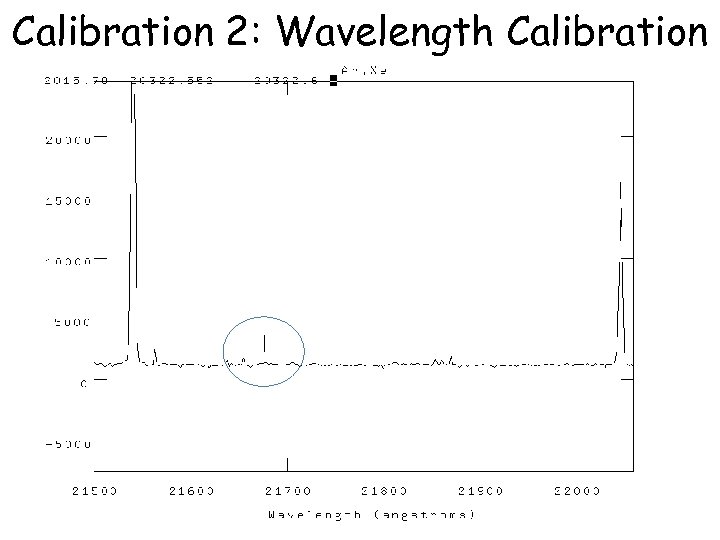
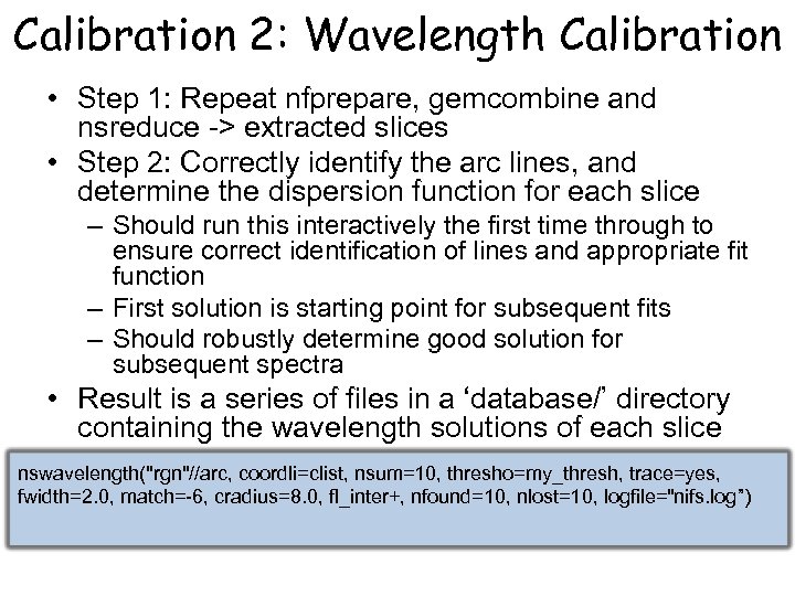Calibration 2: Wavelength Calibration • Step 1: Repeat nfprepare, gemcombine and nsreduce -> extracted slices • Step 2: Correctly identify the arc lines, and determine the dispersion function for each slice – Should run this interactively the first time through to ensure correct identification of lines and appropriate fit function – First solution is starting point for subsequent fits – Should robustly determine good solution for subsequent spectra • Result is a series of files in a ‘database/’ directory containing the wavelength solutions of each slice nswavelength("rgn"//arc, coordli=clist, nsum=10, thresho=my_thresh, trace=yes, fwidth=2. 0, match=-6, cradius=8. 0, fl_inter+, nfound=10, nlost=10, logfile="nifs. log”)

Calibration 2: Wavelength Calibration

Calibration 2: Wavelength Calibration

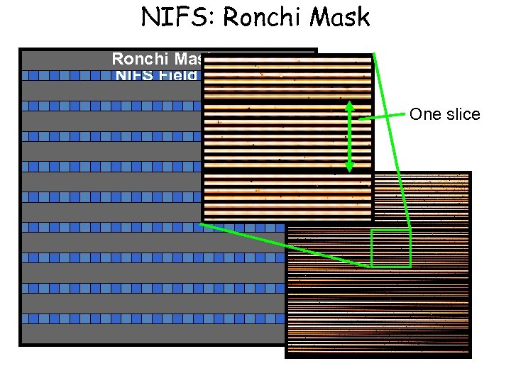
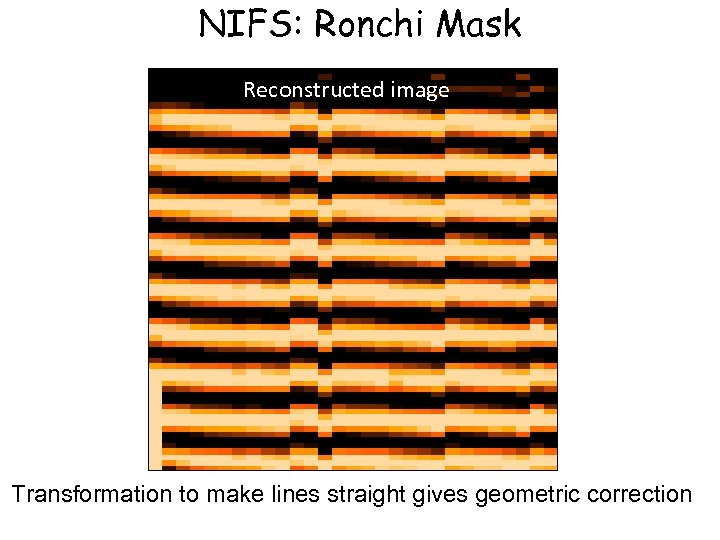
Calibration 3: Spatial Distortion • Need to correct for distortions along the slices, and registration between slices • This is done using the Ronchi mask as a reference • Analogous to wavelength calibration, but in spatial domain

NIFS: Ronchi Mask NIFS Field One slice

NIFS: Ronchi Mask Reconstructed image Transformation to make lines straight gives geometric correction

Calibration 3: Spatial Distortion • Step 1: Repeat nfprepare, gemcombine and nsreduce -> extracted slices • Step 2: run nfsdist – Reference peaks are very regular, so easy to fall foul of aliasing when run automatically – Recommend running interactively for each daycal set nfsdist("rgn"//ronchiflat, fwidth=6. 0, cradius=8. 0, glshift=2. 8, minsep=6. 5, thresh=2000. 0, nlost=3, fl_int+, logfile="nifs. log”) • TIP: apply the distortion correction to the Ronchi frame itself, and check its OK

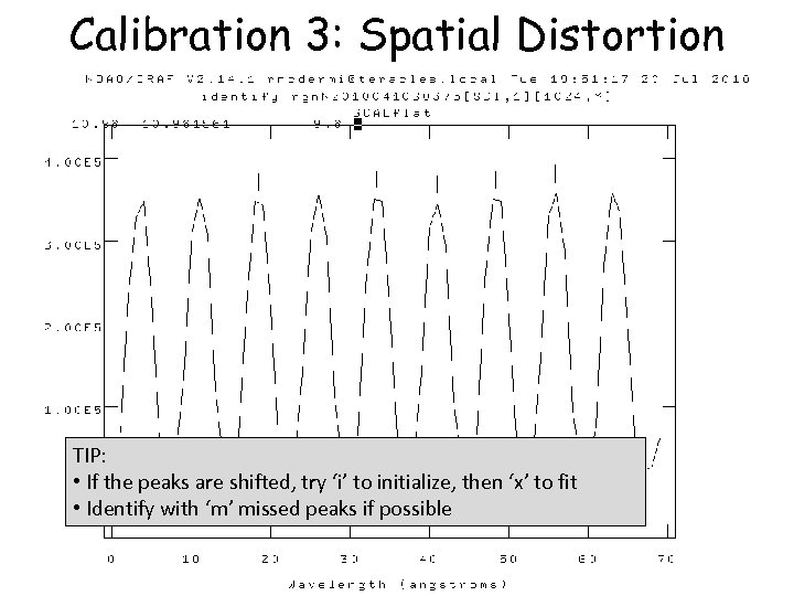Calibration 3: Spatial Distortion TIP: • If the peaks are shifted, try ‘i’ to initialize, then ‘x’ to fit • Identify with ‘m’ missed peaks if possible

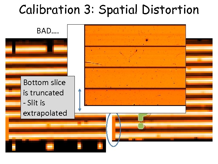Calibration 3: Spatial Distortion BAD…. Bottom slice is truncated - Slit is extrapolated GOOD! ?

Lamp Calibrations: Summary You now have: 1. Shift reference file: "s"+calflat 2. Flat field: "rn"+calflat+"_flat" 3. Flat BPM (for DQ plane generation): "rn"+calflat+"_flat_bpm. pl” 4. Wavelength referenced Arc: "wrn"+arc 5. Spatially referenced Ronchi Flat: "rn"+ronchiflat Notes: – – – 1 -3 are files that you need 4 & 5 are files with associated files in the ‘database/’ dir Arcs are likely together with science data

Telluric Star • Similar to science reduction up to a point: – Sky subtraction – Spectra extraction => 3 D – Wavelength calibration – Flat fielding • Then extract 1 D spectra, co-add separate observations, and derive the telluric correction spectrum

Telluric Star • Preliminaries: – Copy the calibration files you will need into telluric directory: – – – Shift file Flat Bad pixel mask (BPM) Ronchi mask + database dir+files Arc file + database dir+files – Make two files listing filenames with (‘object’) and without (‘sky’) star in field

Telluric Star • Step 1. 1: Run nfprepare, making use of the shift file and BPM • Step 1. 2: Combine the blank sky frames: – Skies are close in time – Use gemcombine and your list of sky frames to create a median sky • Step 1. 3: Subtract the combined sky from each object frame with gemarith

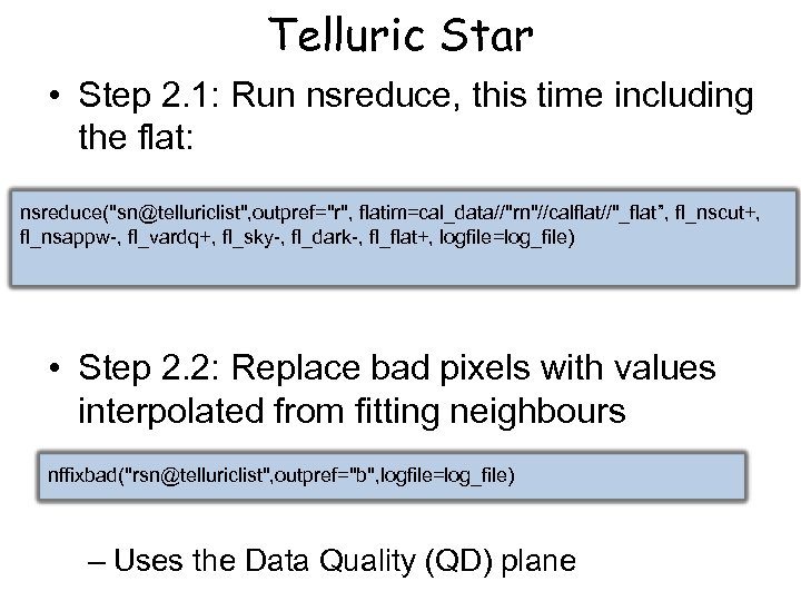Telluric Star • Step 2. 1: Run nsreduce, this time including the flat: nsreduce("sn@telluriclist", outpref="r", flatim=cal_data//"rn"//calflat//"_flat”, fl_nscut+, fl_nsappw-, fl_vardq+, fl_sky-, fl_dark-, fl_flat+, logfile=log_file) • Step 2. 2: Replace bad pixels with values interpolated from fitting neighbours nffixbad("rsn@telluriclist", outpref="b", logfile=log_file) – Uses the Data Quality (QD) plane

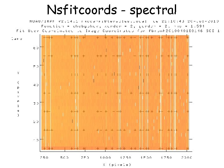
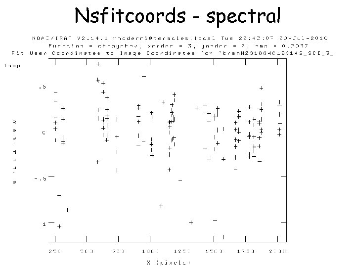
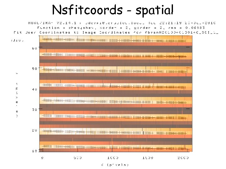
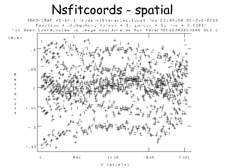
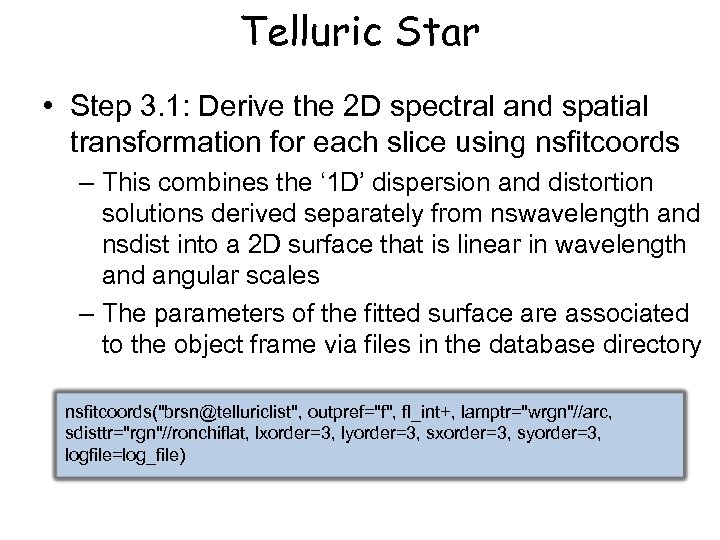Telluric Star • Step 3. 1: Derive the 2 D spectral and spatial transformation for each slice using nsfitcoords – This combines the ‘ 1 D’ dispersion and distortion solutions derived separately from nswavelength and nsdist into a 2 D surface that is linear in wavelength and angular scales – The parameters of the fitted surface are associated to the object frame via files in the database directory nsfitcoords("brsn@telluriclist", outpref="f", fl_int+, lamptr="wrgn"//arc, sdisttr="rgn"//ronchiflat, lxorder=3, lyorder=3, sxorder=3, syorder=3, logfile=log_file)

Nsfitcoords - spectral

Nsfitcoords - spectral

Nsfitcoords - spatial

Nsfitcoords - spatial

Telluric Star • Step 3. 2: Transform the slice images to the linear physical coordinates using nstransform – Uses transforms defined by nsfitcoords – Generates slices that are sampled in constant steps of wavelength and arcsec • This is essentially a data-cube (even though its not a cube…) – Can run analysis directly from this point

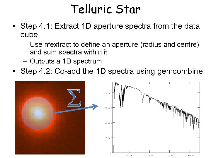Telluric Star • Step 4. 1: Extract 1 D aperture spectra from the data cube – Use nfextract to define an aperture (radius and centre) and sum spectra within it – Outputs a 1 D spectrum • Step 4. 2: Co-add the 1 D spectra using gemcombine

Science Data • Same preliminaries as telluric: – Copy database and arc+Ronchi files – Copy shift file, flat and BPM – Identify sky and object frames • In addition, we make use of the 1 D telluric • Generally need to combine separate (and dithered) data-cubes

Science Data • Initial steps: – Nfprepare as per telluric – Subtract sky using gemarith • Usually have one unique sky per object: ABAB • Can have ABA – two science share a sky – Nsreduce (inc. flat field) – Nffixbad, nsfitcoords, nstransform • Now have data-cube with linear physical coordinates

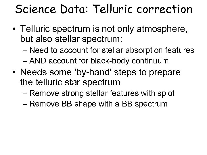Science Data: Telluric correction • Telluric spectrum is not only atmosphere, but also stellar spectrum: – Need to account for stellar absorption features – AND account for black-body continuum • Needs some ‘by-hand’ steps to prepare the telluric star spectrum – Remove strong stellar features with splot – Remove BB shape with a BB spectrum

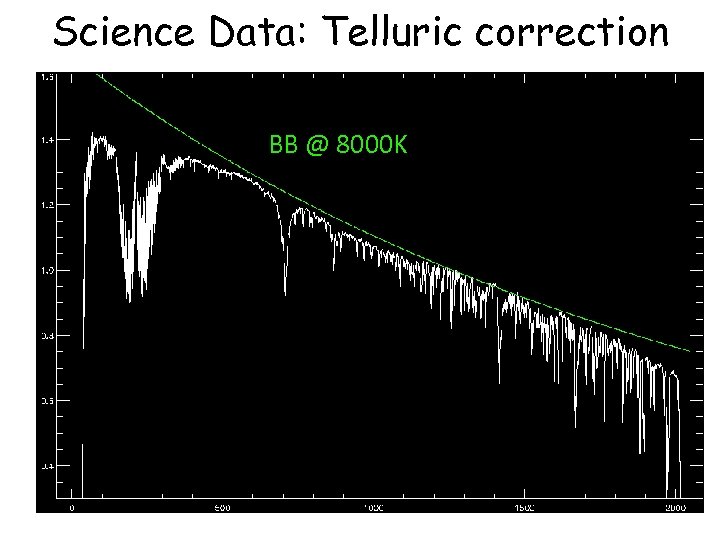Science Data: Telluric correction BB @ 8000 K

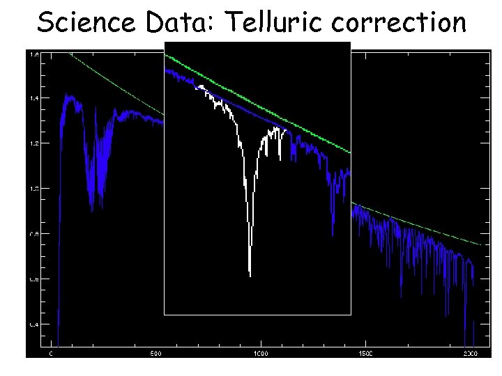Science Data: Telluric correction BB @ 8000 K

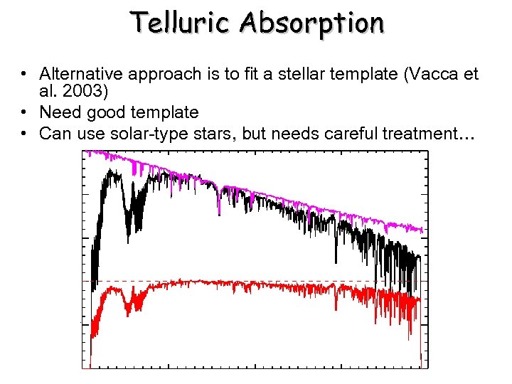Telluric Absorption • Alternative approach is to fit a stellar template (Vacca et al. 2003) • Need good template • Can use solar-type stars, but needs careful treatment…

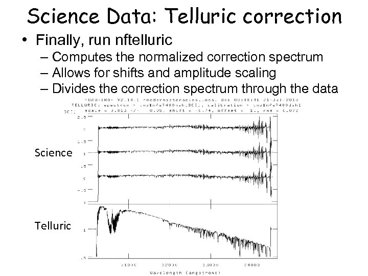Science Data: Telluric correction • Finally, run nftelluric – Computes the normalized correction spectrum – Allows for shifts and amplitude scaling – Divides the correction spectrum through the data Science Telluric

Science Data: Merging • Now have series of data-cubes: – No dark current or sky (sky-subtracted) – Spatially and spectrally linearized – Bad pixels interpolated over – No instrumental transmission (flat-fielded) – No atmospheric transmission (telluric-corrected) • Need to combine the data-cubes • Will do this in three steps: – Convert MEF ‘cubes’ to real 3 D arrays – Determine the relative spatial origin and adapt the WCS headers – Use gemcube to combine the cubes

Science Data: Merging • Use nfcube to create the 3 D arrays – Uses interpolation to go from series of 2 D slices to one rectilinear 3 D array – Default pixel scale is 0. 05”x 0. 05” (arrays need square pixels. . ) • These cubes are easily displayed using ds 9 – Load as an array, scroll through the slices • Find a reference pixel coordinate – Should be easily recognizable in the cube – Should be common to all cubes • Adapt the headers to reflect the common spatial axes origin • Run gemcube

Science Data: Merging • This approach involves (at least) one superfluous interpolation: nifcube + gemcube both interpolate • Might be possible to use gemcube directly from transformed data, but may need wrapper (TBD: works on single slices, so can be adapted) • Nifcube step is convenient for determining reference coordinate • At least gives a way to combine your data at this point – stay tuned for updated documentation