News and Notes 4 8 HW 3 due

News and Notes 4/8 • HW 3 due date delayed to Tuesday 4/13 – will hand out HW 4 on 4/13 also • Today: finish up NW economics • Tuesday 4/13 – another mandatory class exercise – topic: evolutionary game theory

Market Economies and Networks Networked Life CSE 112 Spring 2004 Prof. Michael Kearns

Market Economies • Suppose there a bunch of different goods – wheat, rice, paper, raccoon pelts, matches, grain alcohol, … – no differences or distinctions within a good: rice is rice • We may all have different initial amounts or endowments – I might have 10 sacks of rice and two raccoon pelts – you might have 6 bushels of wheat, 2 boxes of matches – etc. • Of course, we may want to exchange some of our goods – I can’t eat 10 sacks of rice, and I need matches to light a fire – it’s getting cold and you need raccoon mittens – etc. • How should we engage in exchange? • What should be the rates of exchange? • These are among the oldest questions in economics

Cash and Prices • Suppose we introduce an abstract good called cash – no inherent value – simply meant to facilitate trade, encode exchange rates • And now suppose we introduce prices in cash – i. e. rates of exchange between each “real” good and cash • Then if we all believed in cash and the prices… – we might try to sell our initial endowments for cash – then use the cash to buy exactly what we most want • But will there really be: – others who want to buy all of our endowments? (demand) – others who will be selling what we want? (supply)

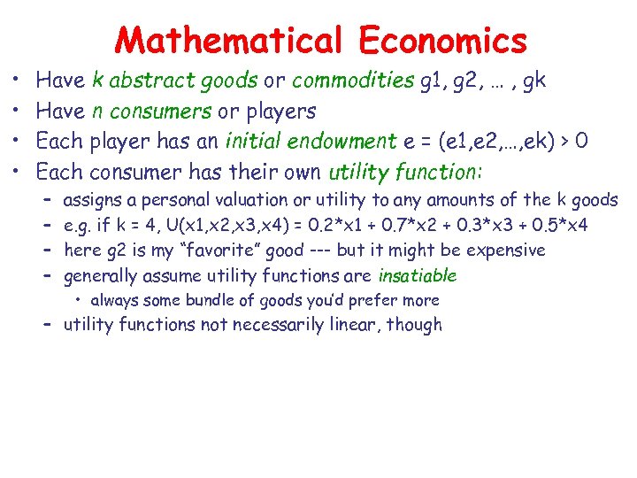Mathematical Economics • • Have k abstract goods or commodities g 1, g 2, … , gk Have n consumers or players Each player has an initial endowment e = (e 1, e 2, …, ek) > 0 Each consumer has their own utility function: – – assigns a personal valuation or utility to any amounts of the k goods e. g. if k = 4, U(x 1, x 2, x 3, x 4) = 0. 2*x 1 + 0. 7*x 2 + 0. 3*x 3 + 0. 5*x 4 here g 2 is my “favorite” good --- but it might be expensive generally assume utility functions are insatiable • always some bundle of goods you’d prefer more – utility functions not necessarily linear, though

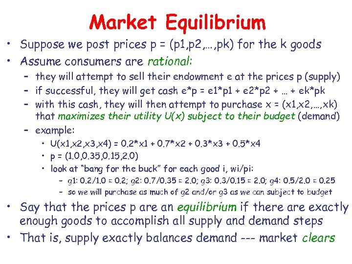Market Equilibrium • Suppose we post prices p = (p 1, p 2, …, pk) for the k goods • Assume consumers are rational: – they will attempt to sell their endowment e at the prices p (supply) – if successful, they will get cash e*p = e 1*p 1 + e 2*p 2 + … + ek*pk – with this cash, they will then attempt to purchase x = (x 1, x 2, …, xk) that maximizes their utility U(x) subject to their budget (demand) – example: • U(x 1, x 2, x 3, x 4) = 0. 2*x 1 + 0. 7*x 2 + 0. 3*x 3 + 0. 5*x 4 • p = (1. 0, 0. 35, 0. 15, 2. 0) • look at “bang for the buck” for each good i, wi/pi: – g 1: 0. 2/1. 0 = 0. 2; g 2: 0. 7/0. 35 = 2. 0; g 3: 0. 3/0. 15 = 2. 0; g 4: 0. 5/2. 0 = 0. 25 – so we will purchase as much of g 2 and/or g 3 as we can subject to budget • Say that the prices p are an equilibrium if there are exactly enough goods to accomplish all supply and demand steps • That is, supply exactly balances demand --- market clears

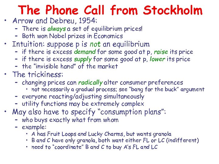The Phone Call from Stockholm • Arrow and Debreu, 1954: – There is always a set of equilibrium prices! – Both won Nobel prizes in Economics • Intuition: suppose p is not an equilibrium – if there is excess demand for some good at p, raise its price – if there is excess supply for some good at p, lower its price – the “invisible hand” of the market • The trickiness: – changing prices can radically alter consumer preferences • not necessarily a gradual process; see “bang for the buck” argument – everyone reacting/adjusting simultaneously – utility functions may be extremely complex • May also have to specify “consumption plans”: – who buys exactly what from whom – example: • A has Fruit Loops and Lucky Charms, but wants granola • B and C have only granola, both want either FL or LC (indifferent) • need to “coordinate” B and C to buy A’s FL and LC

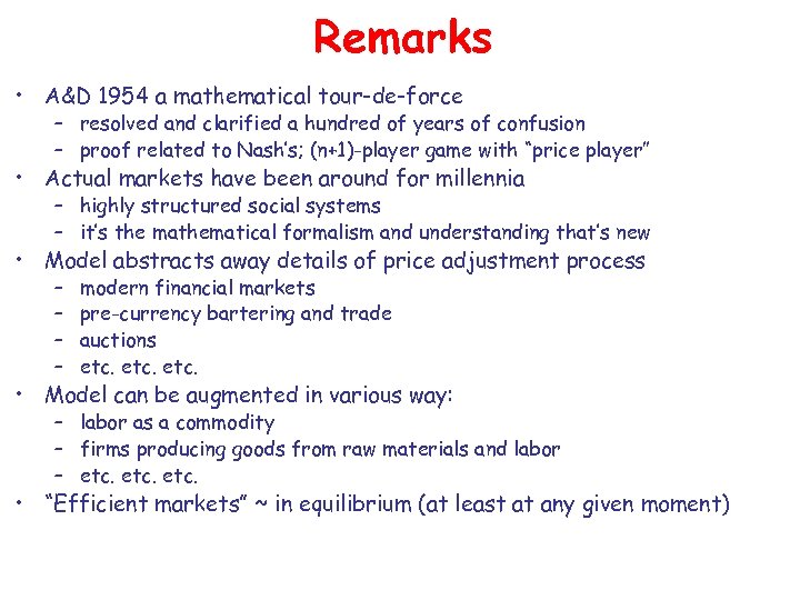Remarks • A&D 1954 a mathematical tour-de-force – resolved and clarified a hundred of years of confusion – proof related to Nash’s; (n+1)-player game with “price player” • Actual markets have been around for millennia – highly structured social systems – it’s the mathematical formalism and understanding that’s new • Model abstracts away details of price adjustment process – – modern financial markets pre-currency bartering and trade auctions etc. • Model can be augmented in various way: – labor as a commodity – firms producing goods from raw materials and labor – etc. • “Efficient markets” ~ in equilibrium (at least at any given moment)

Network Economics • All of what we’ve said so far assumes: – – that anyone can trade (buy or sell) with anyone else wheat bought from Nick is the same as wheat bought from Kilian equivalently, exchange takes place on a complete network global prices must emerge due to competition • But there are many economic settings in which everyone is not free to trade with everyone else – geography: • perishability: you buy groceries from local markets so it won’t spoil • labor: you purchases services from local residents – legality: • if one were to purchase drugs, it is likely to be from an acquaintance (no centralized market possible) • peer-to-peer music exchange – politics: • there may be trade embargoes between nations – regulations: • on Wall Street, certain transactions (within a firm) may be prohibited

Next Up • A model of network economics • Analysis of our experiment • Network economics and preferential attachment

A Network Model of Market Economies • Still begin with the same framework: – k goods or commodities – n consumers, each with their own endowments and utility functions • But now assume an undirected network dictating exchange – each vertex is a consumer – edge between i and j means they are free to engage in trade – no edge between i and j: direct exchange is forbidden • Note: can “encode” network in goods and utilities – for each raw good g and consumer i, introduce virtual good (g, i) – think of (g, i) as “good g when sold by consumer i” – consumer j will have • zero utility for (g, i) if no edge between i and j • j’s original utility for g if there is an edge between i and j

Network Equilibrium • Now prices are for each (g, i), not for just raw goods – permits the possibility of variation in price for raw goods – prices of (g, i) and (g, j) may differ – what would cause such variation at equilibrium? • Each consumer must still behave rationally – attempt to sell all of initial endowment, but only to NW neighbors – attempt to purchase goods maximizing utility within budget – will only purchase g from those neighbors with minimum price for g • Market equilibrium still always exists! – set of prices (and consumptions plans) such that: • all initial endowments sold (no excess supply) • no consumer has money left over (no excess demand)

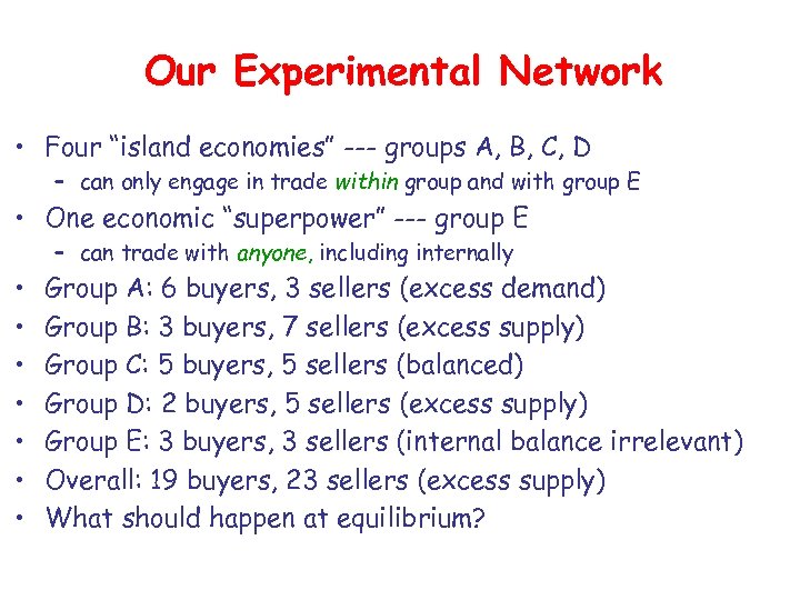Our Experimental Network • Four “island economies” --- groups A, B, C, D – can only engage in trade within group and with group E • One economic “superpower” --- group E – can trade with anyone, including internally • • Group A: 6 buyers, 3 sellers (excess demand) Group B: 3 buyers, 7 sellers (excess supply) Group C: 5 buyers, 5 sellers (balanced) Group D: 2 buyers, 5 sellers (excess supply) Group E: 3 buyers, 3 sellers (internal balance irrelevant) Overall: 19 buyers, 23 sellers (excess supply) What should happen at equilibrium?

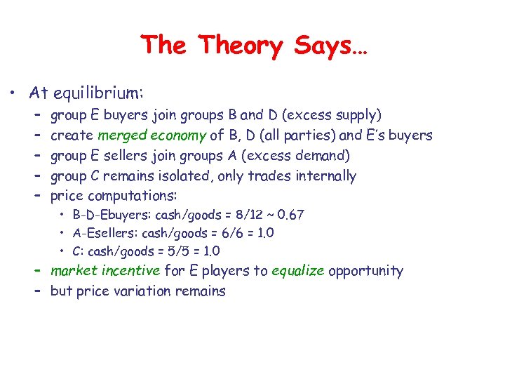The Theory Says… • At equilibrium: – – – group E buyers join groups B and D (excess supply) create merged economy of B, D (all parties) and E’s buyers group E sellers join groups A (excess demand) group C remains isolated, only trades internally price computations: • B-D-Ebuyers: cash/goods = 8/12 ~ 0. 67 • A-Esellers: cash/goods = 6/6 = 1. 0 • C: cash/goods = 5/5 = 1. 0 – market incentive for E players to equalize opportunity – but price variation remains

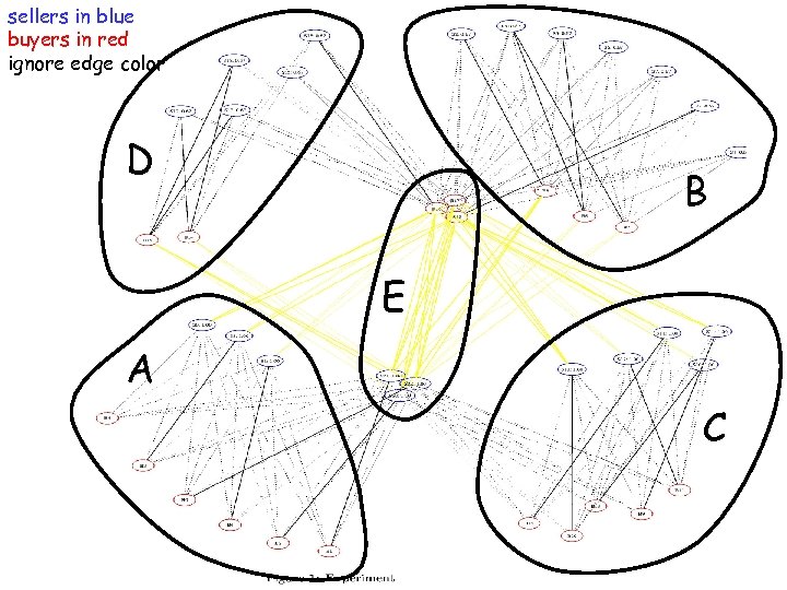sellers in blue buyers in red ignore edge color D B E A C

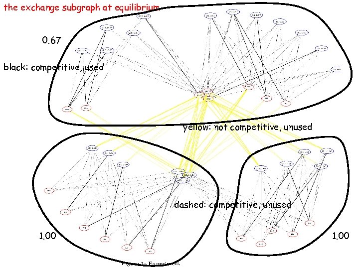the exchange subgraph at equilibrium 0. 67 black: competitive, used yellow: not competitive, unused dashed: competitive, unused 1. 00

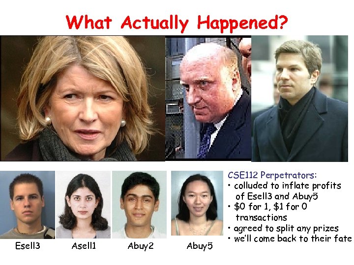What Actually Happened? Esell 3 Asell 1 Abuy 2 Abuy 5 CSE 112 Perpetrators: • colluded to inflate profits of Esell 3 and Abuy 5 • $0 for 1, $1 for 0 transactions • agreed to split any prizes • we’ll come back to their fate

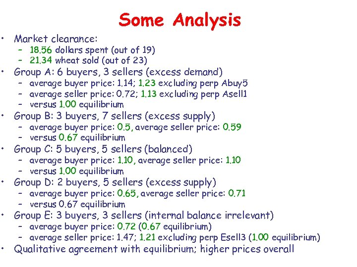Some Analysis • Market clearance: – 18. 56 dollars spent (out of 19) – 21. 34 wheat sold (out of 23) • Group A: 6 buyers, 3 sellers (excess demand) – average buyer price: 1. 14; 1. 23 excluding perp Abuy 5 – average seller price: 0. 72; 1. 13 excluding perp Asell 1 – versus 1. 00 equilibrium • Group B: 3 buyers, 7 sellers (excess supply) – average buyer price: 0. 5, average seller price: 0. 59 – versus 0. 67 equilibrium • Group C: 5 buyers, 5 sellers (balanced) – average buyer price: 1. 10, average seller price: 1. 10 – versus 1. 00 equilibrium • Group D: 2 buyers, 5 sellers (excess supply) – average buyer price: 0. 65, average seller price: 0. 71 – versus 0. 67 equilibrium • Group E: 3 buyers, 3 sellers (internal balance irrelevant) – average buyer price: 0. 72 (0. 67 equilibrium) – average seller price: 1. 47; 1. 21 excluding perp Esell 3 (1. 00 equilibrium) • Qualitative agreement with equilibrium; higher prices overall

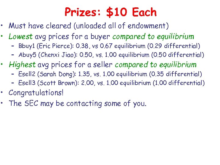Prizes: $10 Each • Must have cleared (unloaded all of endowment) • Lowest avg prices for a buyer compared to equilibrium – Bbuy 1 (Eric Pierce): 0. 38, vs 0. 67 equilibrium (0. 29 differential) – Abuy 5 (Chenxi Jiao): 0. 50, vs. 1. 00 equilibrium (0. 50 differential) • Highest avg prices for a seller compared to equilibrium – Esell 2 (Sarah Dong): 1. 35, vs. 1. 00 equilibrium (0. 35 differential) – Esell 3 (Scott Brown): 2. 00, vs. 1. 00 equilibrium (1. 00 differential) • Congratulations! • The SEC may be contacting some of you.

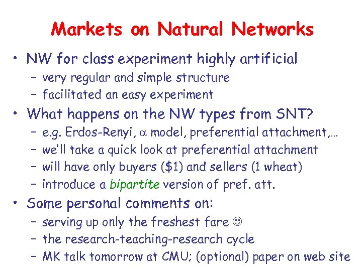Markets on Natural Networks • NW for class experiment highly artificial – very regular and simple structure – facilitated an easy experiment • What happens on the NW types from SNT? – – e. g. Erdos-Renyi, a model, preferential attachment, … we’ll take a quick look at preferential attachment will have only buyers ($1) and sellers (1 wheat) introduce a bipartite version of pref. att. • Some personal comments on: – serving up only the freshest fare – the research-teaching-research cycle – MK talk tomorrow at CMU; (optional) paper on web site

A Preferential Attachment Model for Buyer-Seller Networks • • Probabilistically generates a bipartite graph Buyers and sellers added in pairs at each time step All edges between buyers and sellers Each new party will have n > 1 links back to extant graph – note: n = 1 generates bipartite trees – larger n generates cyclical graphs • Distribution of new buyer’s links: – with prob. 1 – a: extant seller chosen w. r. t. preferential attachment – with prob. a: extant seller chosen uniformly at random – a = 0 is pure pref. att. ; a = 1 is “like” Erdos-Renyi model • So (a, n) characterizes distribution of generative model

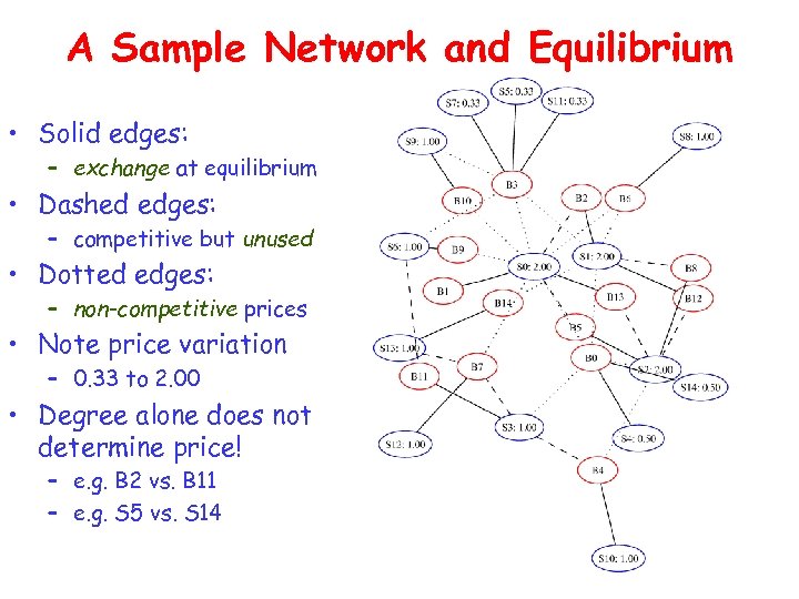A Sample Network and Equilibrium • Solid edges: – exchange at equilibrium • Dashed edges: – competitive but unused • Dotted edges: – non-competitive prices • Note price variation – 0. 33 to 2. 00 • Degree alone does not determine price! – e. g. B 2 vs. B 11 – e. g. S 5 vs. S 14

Basic Theory

Statistics of the Network • Can generate standard range of degree distributions • Define b = (1 -a)n/(1+n) – varies from (1 -a)/2 to 1 -a • Theorem: in the (a, n) model, for x = o(n^(1/b)), the fraction of sellers at time n with degree > x is Q(x^(-1/b)). – closely follows standard techniques – (a = 0, n = 1) yields cumulative distribution Q(x^(-2)) – as a 1, tails become lighter; exponential decay at a = 1

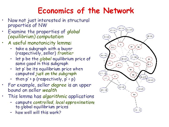Economics of the Network • Now not just interested in structural properties of NW • Examine the properties of global (equilibrium) computation • A useful monotonicity lemma: – take a subgraph with a buyer (respectively, seller) frontier – let p be the global equilibrium price of some good in this subgraph – let p’ be its equilibrium price when computed just on the subgraph – then p’ > p (respectively, p’ < p) • For example, seller degree is an upper bound on seller wealth • This lemma has algorithmic applications – compute controlled, local approximations to global equilibrium prices – how well will this work?

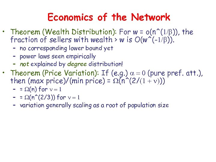Economics of the Network • Theorem (Wealth Distribution): For w = o(n^(1/b)), the fraction of sellers with wealth > w is O(w^(-1/b)). – no corresponding lower bound yet – power laws seen empirically – not explained by degree distribution! • Theorem (Price Variation): If (e. g. ) a = 0 (pure pref. att. ), then (max price)/(min price) = W(n^(2/(1 + n))) – = W(n) for n = 1 – = W(n^(2/3)) for n = 1 – variation generally scaling as a root of population size

Simulation Studies

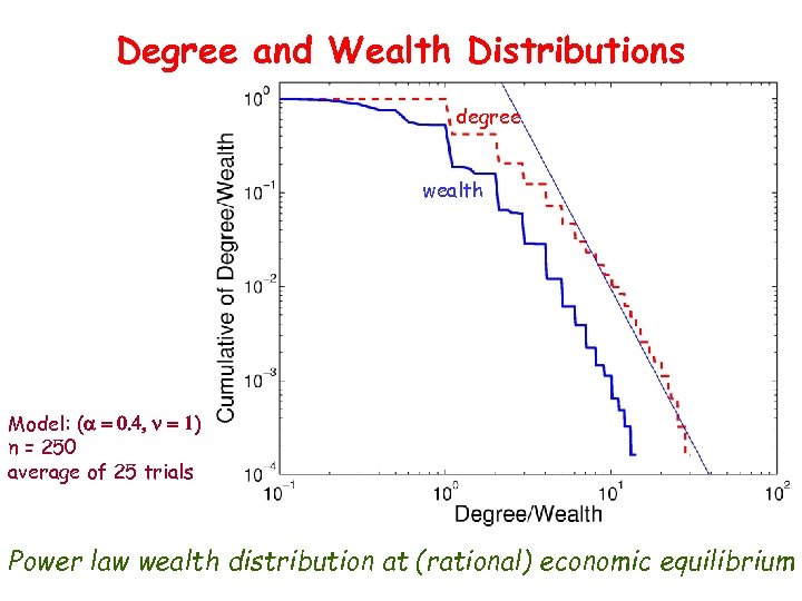Degree and Wealth Distributions degree wealth Model: (a = 0. 4, n = 1) n = 250 average of 25 trials Power law wealth distribution at (rational) economic equilibrium

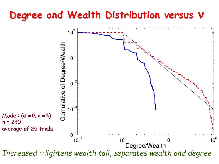Degree and Wealth Distribution versus n Model: (a = 0, n = 2) n = 250 average of 25 trials Increased n lightens wealth tail, separates wealth and degree

Price Variation vs. NW Size & n Model: (a = 0, n varying) average of 25 trials Power of network size (matches theory); decreasing with n

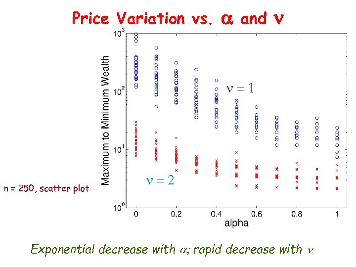Price Variation vs. a and n n=1 n = 250, scatter plot n=2 Exponential decrease with a; rapid decrease with n

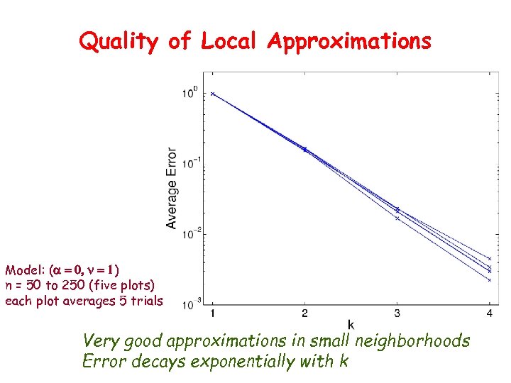Quality of Local Approximations Model: (a = 0, n = 1) n = 50 to 250 (five plots) each plot averages 5 trials Very good approximations in small neighborhoods Error decays exponentially with k

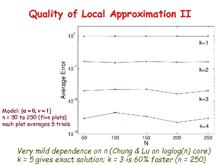Quality of Local Approximation II Model: (a = 0, n = 1) n = 50 to 250 (five plots) each plot averages 5 trials Very mild dependence on n (Chung & Lu on loglog(n) core) k = 5 gives exact solution; k = 3 is 60% faster (n = 250)