New Product Decision Models G Product design using

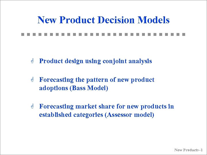New Product Decision Models G Product design using conjoint analysis G Forecasting the pattern of new product adoptions (Bass Model) G Forecasting market share for new products in established categories (Assessor model) New Products– 1

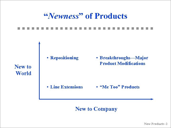“Newness” of Products • Repositioning • Breakthroughs—Major Product Modifications • Line Extensions • “Me Too” Products New to World New to Company New Products– 2

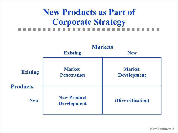New Products as Part of Corporate Strategy Markets Existing New Market Penetration Market Development New Product Development (Diversification) Products New Products– 3

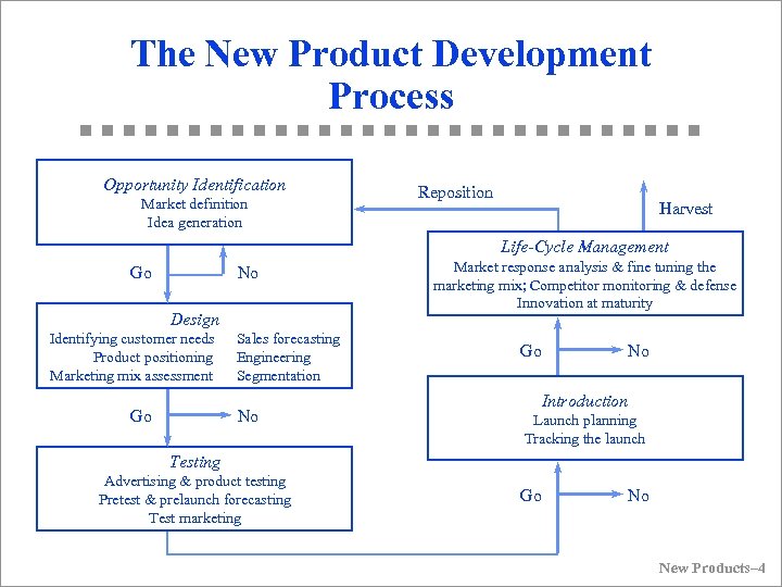The New Product Development Process Opportunity Identification Market definition Idea generation Reposition Harvest Life-Cycle Management Go No Design Identifying customer needs Product positioning Marketing mix assessment Go Sales forecasting Engineering Segmentation No Market response analysis & fine tuning the marketing mix; Competitor monitoring & defense Innovation at maturity Go No Introduction Launch planning Tracking the launch Testing Advertising & product testing Pretest & prelaunch forecasting Test marketing Go No New Products– 4

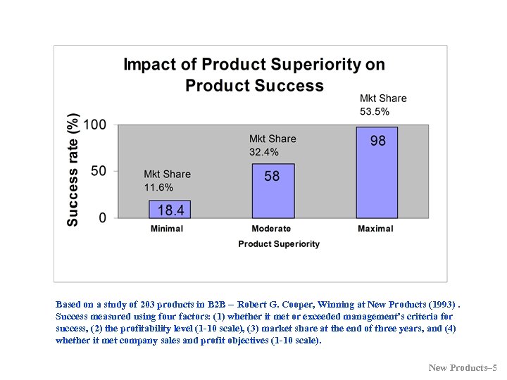Based on a study of 203 products in B 2 B -- Robert G. Cooper, Winning at New Products (1993). Success measured using four factors: (1) whether it met or exceeded management’s criteria for success, (2) the profitability level (1 -10 scale), (3) market share at the end of three years, and (4) whether it met company sales and profit objectives (1 -10 scale). New Products– 5

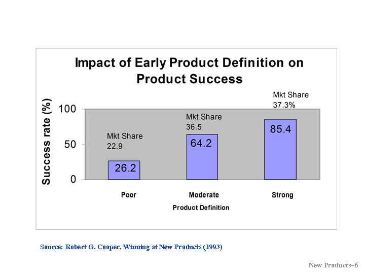Source: Robert G. Cooper, Winning at New Products (1993) New Products– 6

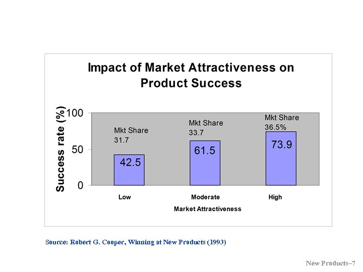Source: Robert G. Cooper, Winning at New Products (1993) New Products– 7

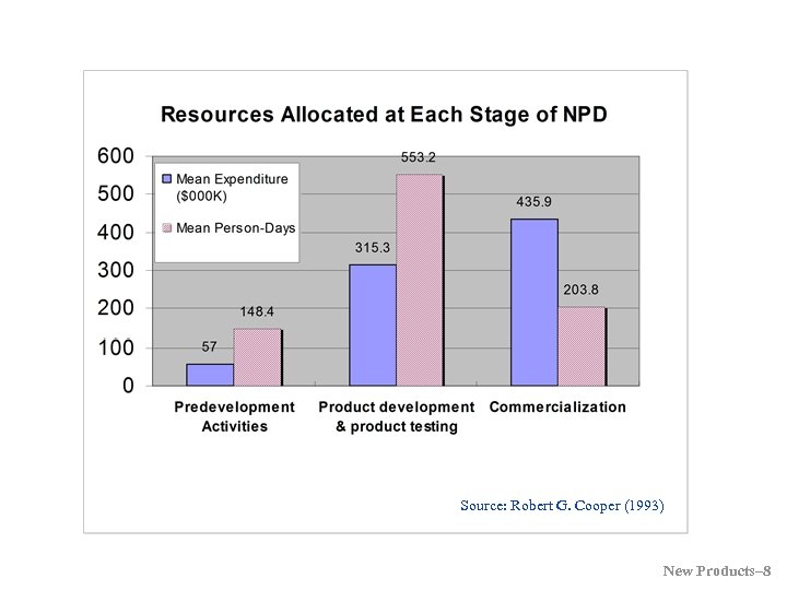Source: Robert G. Cooper (1993) New Products– 8

Value of Good Design 80% of a product’s manufacturing costs are incurred during the first 20% of its design (varies with product category). Conjoint Analysis is a systematic approach for matching product design with the needs and wants of customers, especially in the early stages of the New Product Development process. Source: Mckinsey & Company Report New Products– 9

What is Conjoint Analysis? A way to understand incorporate the structure of customer preferences into the new product design process. In particular, it enables one to evaluate how customers make tradeoffs between various product attributes. The basic output of conjoint analysis are: • A numerical assessment of the relative importance that customers attach to attributes of a product category • The value (utility) provided to customers by each potential feature of a product New Products– 10

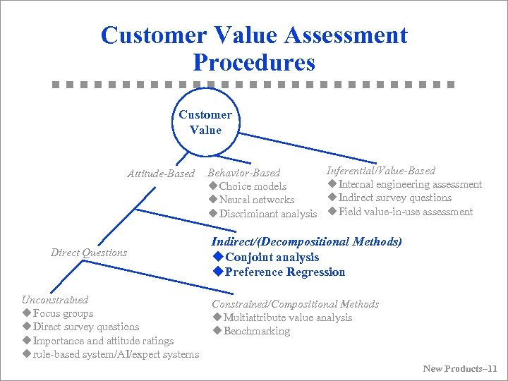Customer Value Assessment Procedures Customer Value Attitude-Based Direct Questions Unconstrained u. Focus groups u. Direct survey questions u. Importance and attitude ratings urule-based system/AI/expert systems Behavior-Based u. Choice models u. Neural networks u. Discriminant analysis Inferential/Value-Based u. Internal engineering assessment u. Indirect survey questions u. Field value-in-use assessment Indirect/(Decompositional Methods) u. Conjoint analysis u. Preference Regression Constrained/Compositional Methods u. Multiattribute value analysis u. Benchmarking New Products– 11

Why is Customer Value Assessment through Conjoint Useful? G Design new products that enhance customer value. G Forecast sales/market share/profit of alternative product concepts. G Identify market segments for which a given concept offers high value. G Identify the “best” concept for a target segment. G Explore impact of alternative pricing and service strategies. G Help production planning in flexible manufacturing systems. New Products– 12

Conjoint Analysis in Product Design Should we offer our business travelers more room space or a fax machine in their room? Given a target cost for a product, should we enhance product reliability or its performance? Should we use a steel or aluminum casing to increase customer preference for the new equipment? New Products– 13

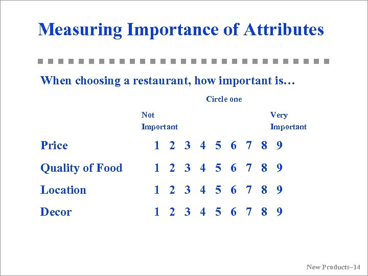Measuring Importance of Attributes When choosing a restaurant, how important is… Circle one Not Important Very Important Price 1 2 3 4 5 6 7 8 9 Quality of Food 1 2 3 4 5 6 7 8 9 Location 1 2 3 4 5 6 7 8 9 Decor 1 2 3 4 5 6 7 8 9 New Products– 14

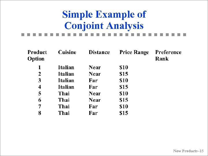Simple Example of Conjoint Analysis New Products– 15

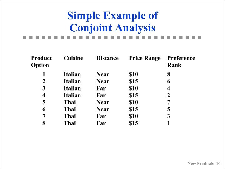Simple Example of Conjoint Analysis New Products– 16

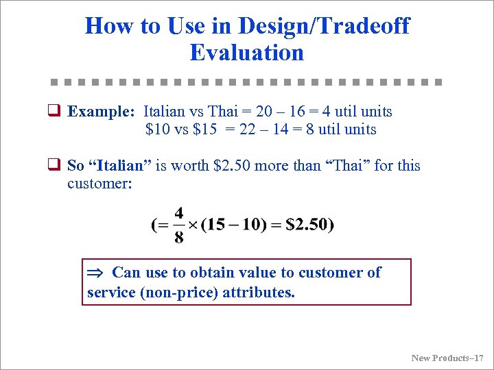How to Use in Design/Tradeoff Evaluation q Example: Italian vs Thai = 20 – 16 = 4 util units $10 vs $15 = 22 – 14 = 8 util units q So “Italian” is worth $2. 50 more than “Thai” for this customer: Þ Can use to obtain value to customer of service (non-price) attributes. New Products– 17

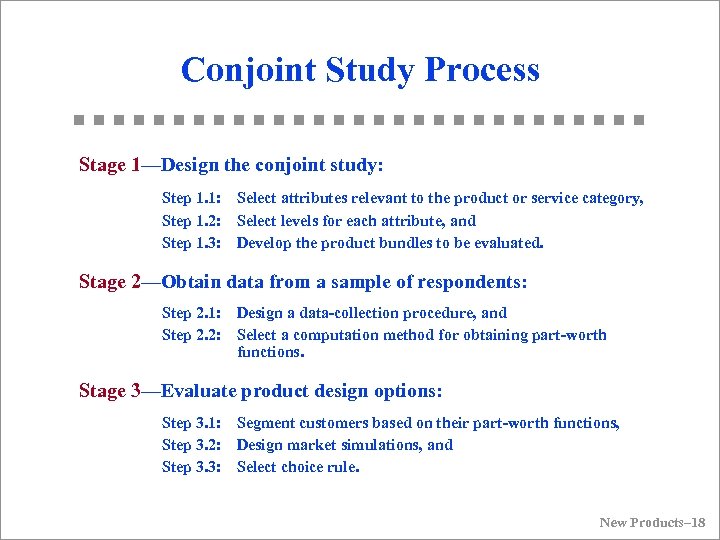Conjoint Study Process Stage 1—Design the conjoint study: Step 1. 1: Select attributes relevant to the product or service category, Step 1. 2: Select levels for each attribute, and Step 1. 3: Develop the product bundles to be evaluated. Stage 2—Obtain data from a sample of respondents: Step 2. 1: Design a data-collection procedure, and Step 2. 2: Select a computation method for obtaining part-worth functions. Stage 3—Evaluate product design options: Step 3. 1: Segment customers based on their part-worth functions, Step 3. 2: Design market simulations, and Step 3. 3: Select choice rule. New Products– 18

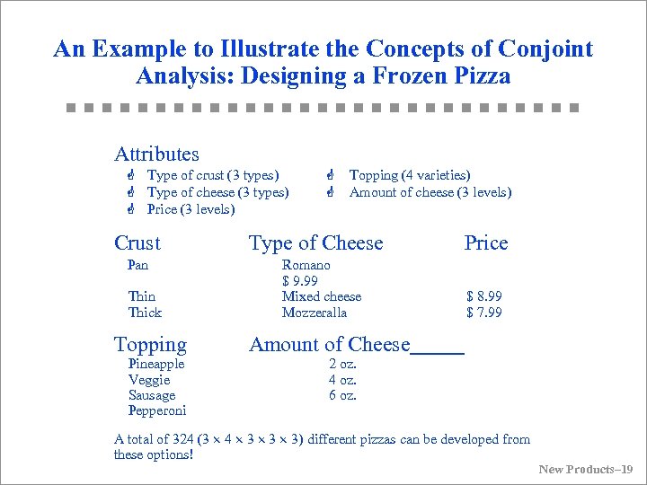An Example to Illustrate the Concepts of Conjoint Analysis: Designing a Frozen Pizza Attributes G Type of crust (3 types) G Type of cheese (3 types) G Price (3 levels) Crust Pan Thick Topping Pineapple Veggie Sausage Pepperoni G Topping (4 varieties) G Amount of cheese (3 levels) Type of Cheese Romano $ 9. 99 Mixed cheese Mozzeralla Price $ 8. 99 $ 7. 99 Amount of Cheese 2 oz. 4 oz. 6 oz. A total of 324 (3 ´ 4 ´ 3 ´ 3) different pizzas can be developed from these options! New Products– 19

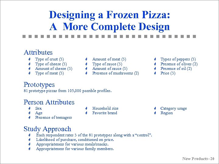Designing a Frozen Pizza: A More Complete Design Attributes G G Type of crust (3) Type of cheese (3) Amount of cheese (3) Type of meat (3) G G Amount of meat (3) Type of sauce (3) Amount of sauce (3) Presence of mushrooms (2) G G Types of peppers (3) Presence of olives (2) Presence of oil (2) Price (3) G G Category usage Region Prototypes 81 prototype pizzas from 105, 000 possible profiles. Person Attributes G G G Sex Age Presence of teenagers G G Household size Favorite brand Study Approach G G Each respondent rates 3 of the 81 prototypes along with a “control”. Likelihood of purchase, conditioned on price. Appropriateness for various meals/snacks. Appropriateness for various family members. New Products– 20

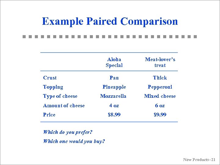Example Paired Comparison Aloha Special Meat-lover’s treat Pan Thick Pineapple Pepperoni Mozzarella Mixed cheese Amount of cheese 4 oz 6 oz Price $8. 99 $9. 99 Crust Topping Type of cheese Which do you prefer? Which one would you buy? New Products– 21

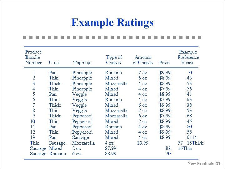Example Ratings Product Bundle Number Crust 1 2 3 4 5 6 7 8 9 10 11 12 13 Thin Sausage Pan Thin Thick Thin Pan Sausage Mixed Romano Topping Type of Cheese Pineapple Veggie Pepperoni Sausage Mozzarella 2 oz 6 oz Romano Mixed Mozzarella Mixed Romano Mixed 4 oz $7. 99 $8. 99 Amount of Cheese 2 oz 6 oz 4 oz 6 oz 2 oz 4 oz $9. 99 Price $9. 99 $8. 99 $7. 99 $8. 99 $9. 99 $8. 99 83 70 Example Preference Score 0 43 53 56 41 63 38 53 68 46 80 58 6114 57 15 Thick 16 Thin New Products– 22

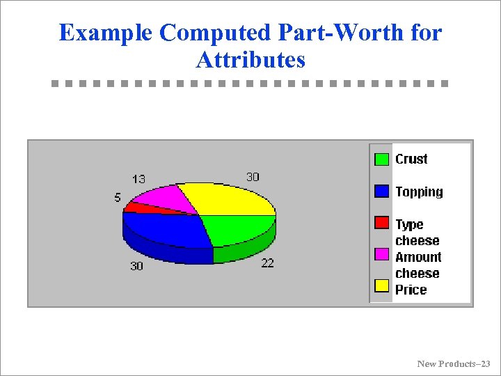Example Computed Part-Worth for Attributes New Products– 23

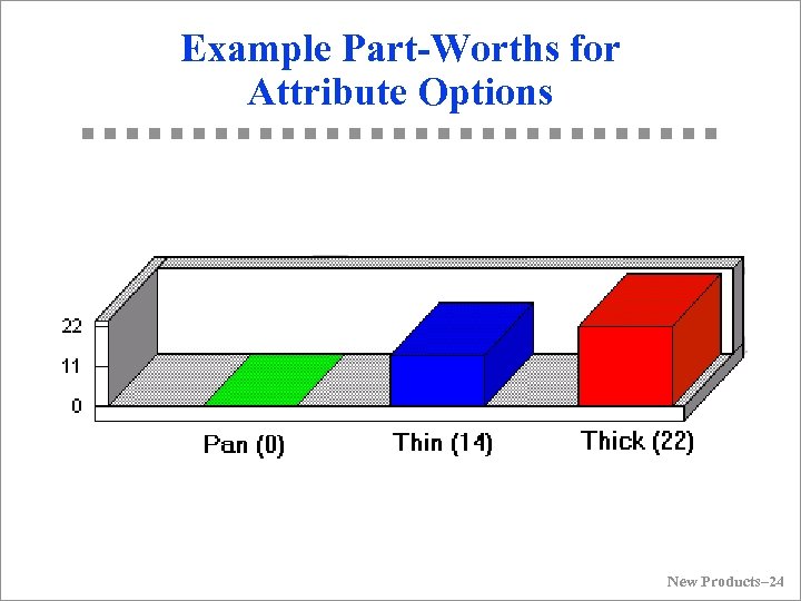Example Part-Worths for Attribute Options New Products– 24

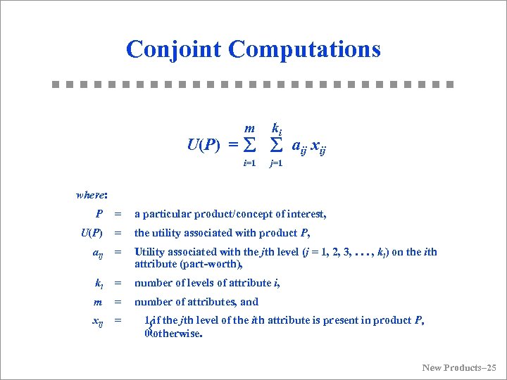Conjoint Computations m ki i=1 j=1 U(P) = å å aij xij where: P = a particular product/concept of interest, U(P) = the utility associated with product P, aij = Utility associated with the jth level (j = 1, 2, 3, . . . , ki) on the ith attribute (part-worth), ki = number of levels of attribute i, m = number of attributes, and xij = { 1 if the jth level of the ith attribute is present in product P, 0 otherwise. New Products– 25

Market Share and Revenue Share Forecasts G Define the competitive set -- these are the products from which the target segment make choices. Some of theses may be existing products and, others concepts being evaluated. We denote this set of products as P 1, P 2, . . . PN. G Select Choice rule u Maximum utility rule u Share of preference rule u Logit choice rule u Alpha rule G Software also has a “Revenue index option” wherein you can compute the revenue index of any product compared to the revenue index of 100 for a base product you select. New Products– 26

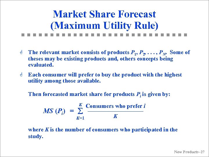Market Share Forecast (Maximum Utility Rule) G The relevant market consists of products P 1, P 2, . . . , PN. Some of theses may be existing products and, others concepts being evaluated. G Each consumer will prefer to buy the product with the highest utility among those available. Then forecasted market share for products Pi is given by: K Consumers who prefer i K=1 K MS (Pi) = å –––––––– where K is the number of consumers who participated in the study. New Products– 27

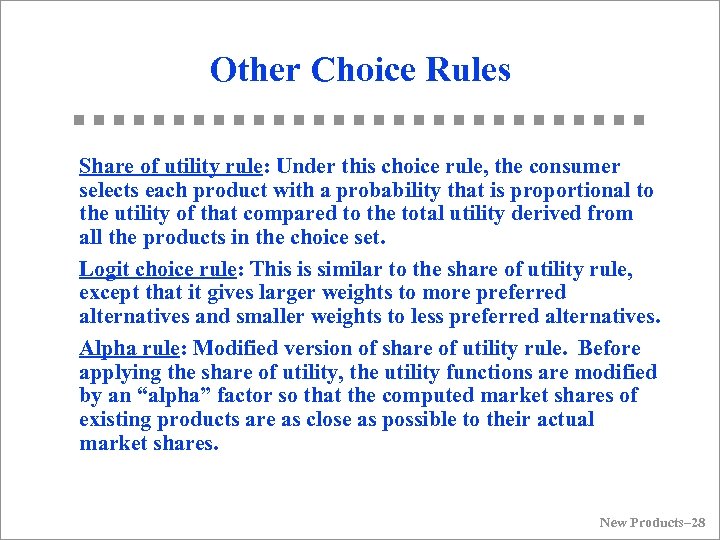Other Choice Rules Share of utility rule: Under this choice rule, the consumer selects each product with a probability that is proportional to the utility of that compared to the total utility derived from all the products in the choice set. Logit choice rule: This is similar to the share of utility rule, except that it gives larger weights to more preferred alternatives and smaller weights to less preferred alternatives. Alpha rule: Modified version of share of utility rule. Before applying the share of utility, the utility functions are modified by an “alpha” factor so that the computed market shares of existing products are as close as possible to their actual market shares. New Products– 28

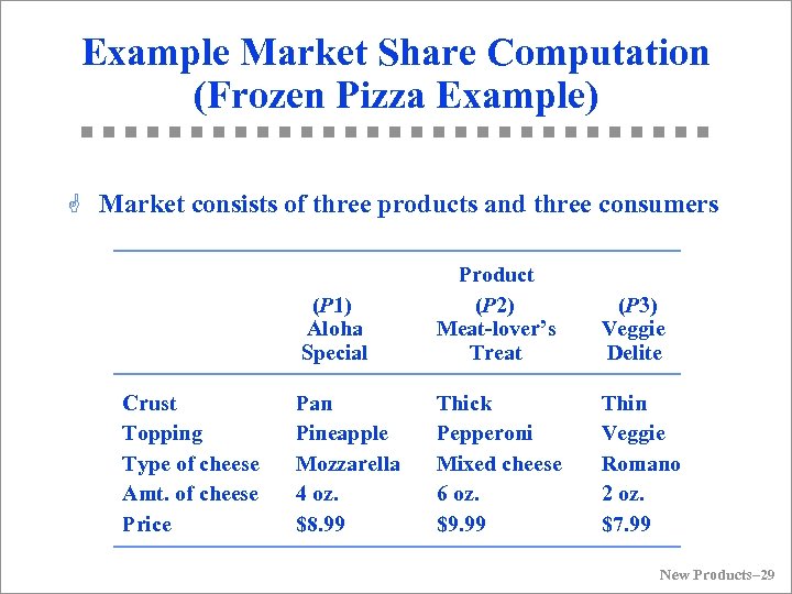Example Market Share Computation (Frozen Pizza Example) G Market consists of three products and three consumers (P 1) Aloha Special Crust Topping Type of cheese Amt. of cheese Price Product (P 2) Meat-lover’s Treat (P 3) Veggie Delite Pan Pineapple Mozzarella 4 oz. $8. 99 Thick Pepperoni Mixed cheese 6 oz. $9. 99 Thin Veggie Romano 2 oz. $7. 99 New Products– 29

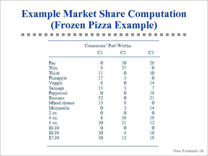Example Market Share Computation (Frozen Pizza Example) Consumers’ Part-Worths Pan Thick Pineapple Veggie Sausage Pepperoni Romano Mixed cheese Mozzarella 2 oz 4 oz. 6 oz. $9. 99 $8. 99 $7. 99 C 1 C 2 C 3 0 9 11 17 6 13 0 52 13 0 0 8 10 0 10 10 10 37 0 3 0 0 9 3 0 39 21 0 4 12 26 0 10 0 14 7 19 21 0 14 0 16 12 0 18 16 New Products– 30

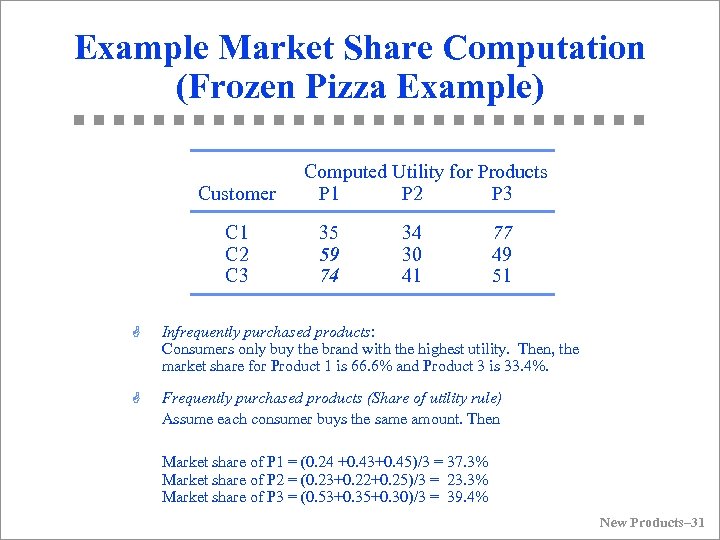Example Market Share Computation (Frozen Pizza Example) Customer C 1 C 2 C 3 Computed Utility for Products P 1 P 2 P 3 35 59 74 34 30 41 77 49 51 G Infrequently purchased products: Consumers only buy the brand with the highest utility. Then, the market share for Product 1 is 66. 6% and Product 3 is 33. 4%. G Frequently purchased products (Share of utility rule) Assume each consumer buys the same amount. Then Market share of P 1 = (0. 24 +0. 43+0. 45)/3 = 37. 3% Market share of P 2 = (0. 23+0. 22+0. 25)/3 = 23. 3% Market share of P 3 = (0. 53+0. 35+0. 30)/3 = 39. 4% New Products– 31

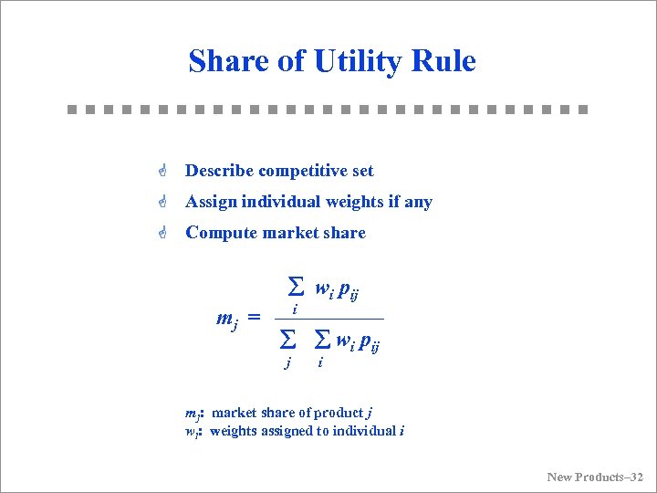Share of Utility Rule G Describe competitive set G Assign individual weights if any G Compute market share å wi pij i mj = ––––– å å wi pij j i mj: market share of product j wi: weights assigned to individual i New Products– 32

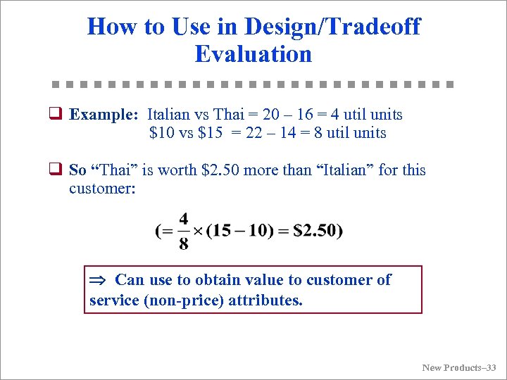How to Use in Design/Tradeoff Evaluation q Example: Italian vs Thai = 20 – 16 = 4 util units $10 vs $15 = 22 – 14 = 8 util units q So “Thai” is worth $2. 50 more than “Italian” for this customer: Þ Can use to obtain value to customer of service (non-price) attributes. New Products– 33

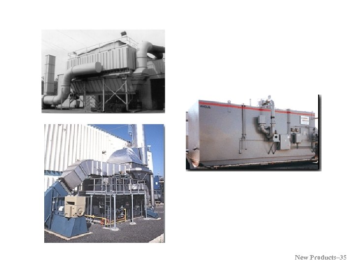
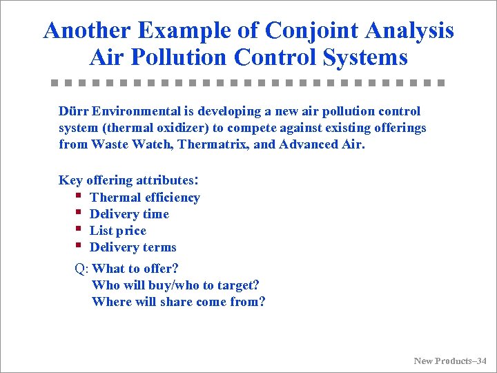Another Example of Conjoint Analysis Air Pollution Control Systems Dürr Environmental is developing a new air pollution control system (thermal oxidizer) to compete against existing offerings from Waste Watch, Thermatrix, and Advanced Air. Key offering attributes: § Thermal efficiency § Delivery time § List price § Delivery terms Q: What to offer? Who will buy/who to target? Where will share come from? New Products– 34

New Products– 35

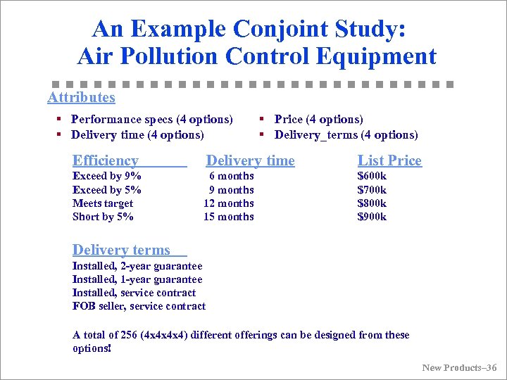An Example Conjoint Study: Air Pollution Control Equipment Attributes § Performance specs (4 options) § Delivery time (4 options) § Price (4 options) § Delivery_terms (4 options) Efficiency Delivery time List Price Exceed by 9% Exceed by 5% Meets target Short by 5% 6 months 9 months 12 months 15 months $600 k $700 k $800 k $900 k Delivery terms Installed, 2 -year guarantee Installed, 1 -year guarantee Installed, service contract FOB seller, service contract A total of 256 (4 x 4 x 4 x 4) different offerings can be designed from these options! New Products– 36

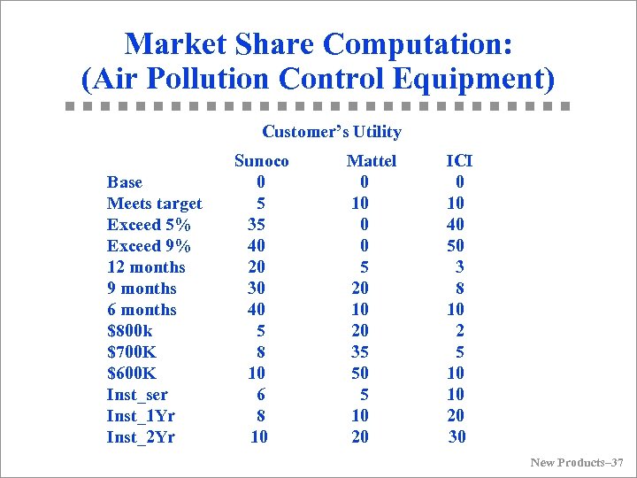Market Share Computation: (Air Pollution Control Equipment) Customer’s Utility Sunoco Base 0 Meets target 5 Exceed 5% 35 Exceed 9% 40 12 months 20 9 months 30 6 months 40 $800 k 5 $700 K 8 $600 K 10 Inst_ser 6 Inst_1 Yr 8 Inst_2 Yr 10 Mattel ICI 0 0 10 0 40 0 5 3 20 8 10 20 2 35 5 50 10 5 10 20 30 New Products– 37

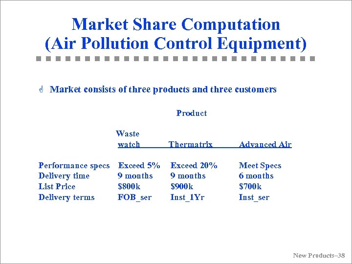Market Share Computation (Air Pollution Control Equipment) G Market consists of three products and three customers Product Waste watch Performance specs Exceed 5% Delivery time 9 months List Price $800 k Delivery terms FOB_ser Thermatrix Advanced Air Exceed 20% 9 months $900 k Inst_1 Yr Meet Specs 6 months $700 k Inst_ser New Products– 38

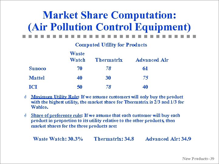Market Share Computation: (Air Pollution Control Equipment) Computed Utility for Products Waste Watch Thermatrix Advanced Air Sunoco 70 78 61 Mattel 40 30 75 ICI 50 78 40 G Maximum Utility Rule: If we assume customers will only buy the product with the highest utility, the market share for Thermatrix is 2/3 and 1/3 for Wahlco. G Share of preference rule: If we assume that each customer will buy each product in proportion to its utility relative to the other products, then market shares for the three products are: Waste Watch: 30. 3% Thermatrix: 34. 8 Advanced Air: 34. 9 New Products– 39

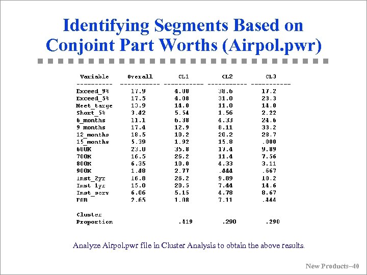Identifying Segments Based on Conjoint Part Worths (Airpol. pwr) Analyze Airpol. pwr file in Cluster Analysis to obtain the above results. New Products– 40

Members in Each Segment 1. Companies in this Segment include u Cummins Engineering, Illinois Tools, Mattel, Neste. Resin, Ralston Purina, New World Technologies, Baltimore Gas, Applied Coatings, Pharmasyn, and Thermal Electric. u These are smaller companies that operate in industries without major pollution problems. They want an equipment that meets EPA efficiency target, medium delivery times, have high price sensitivity, and require installation and warranty. New Products– 41

Members in Each Segment 2. Companies in this Segment include u ICI, Mobil, Maytag, Texaco, Union Carbide, Dow Chemicals, Boise Cascade, and 3 M. u These are large chemical and paper companies that have pollution issues to deal with. They want an equipment that Exceeds EPA efficiency target, have long delivery times (perhaps for installation in new factories that they build), have moderate price sensitivity, and do not require installation help or warranty (FOB). New Products– 42

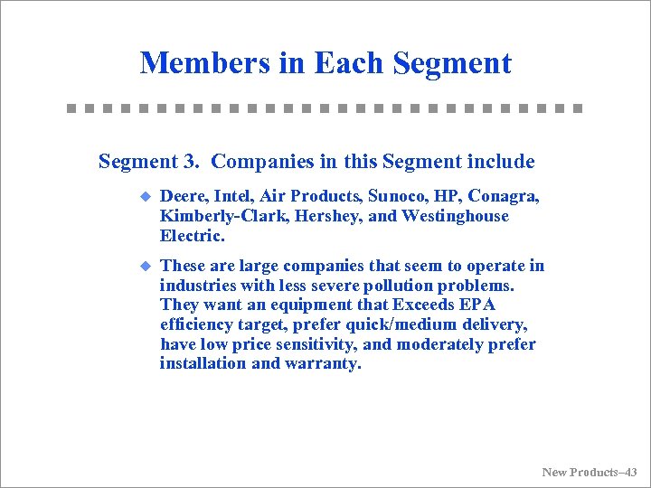Members in Each Segment 3. Companies in this Segment include u Deere, Intel, Air Products, Sunoco, HP, Conagra, Kimberly-Clark, Hershey, and Westinghouse Electric. u These are large companies that seem to operate in industries with less severe pollution problems. They want an equipment that Exceeds EPA efficiency target, prefer quick/medium delivery, have low price sensitivity, and moderately prefer installation and warranty. New Products– 43

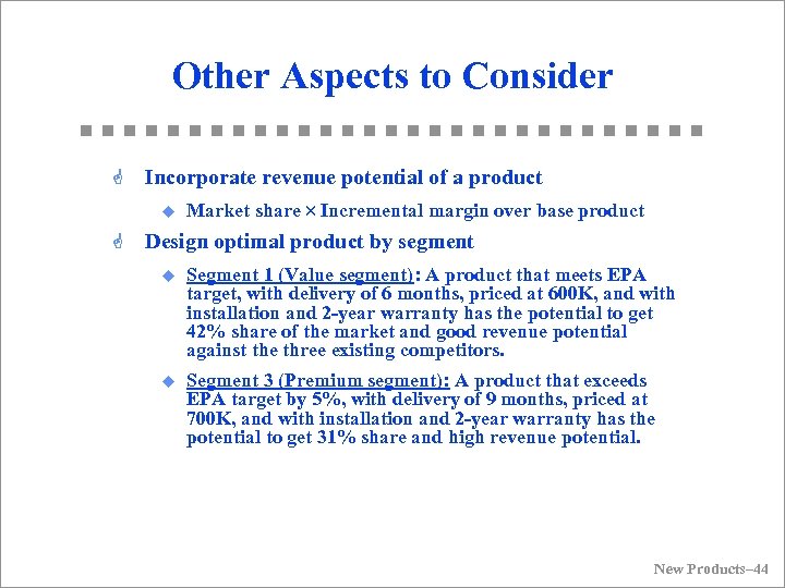Other Aspects to Consider G Incorporate revenue potential of a product u G Market share Incremental margin over base product Design optimal product by segment u Segment 1 (Value segment): A product that meets EPA target, with delivery of 6 months, priced at 600 K, and with installation and 2 -year warranty has the potential to get 42% share of the market and good revenue potential against the three existing competitors. u Segment 3 (Premium segment): A product that exceeds EPA target by 5%, with delivery of 9 months, priced at 700 K, and with installation and 2 -year warranty has the potential to get 31% share and high revenue potential. New Products– 44

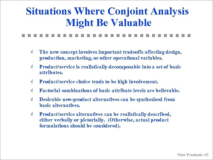Situations Where Conjoint Analysis Might Be Valuable G The new concept involves important tradeoffs affecting design, production, marketing, or other operational variables. G Product/service is realistically decomposable into a set of basic attributes. G Product/service choice tends to be high involvement. G Factorial combinations of basic attribute levels are believable. G Desirable new-product alternatives can be synthesized from basic alternatives. G Product/service alternatives can be realistically described, either verbally or pictorially. (Otherwise, actual product formulations should be considered). New Products– 45

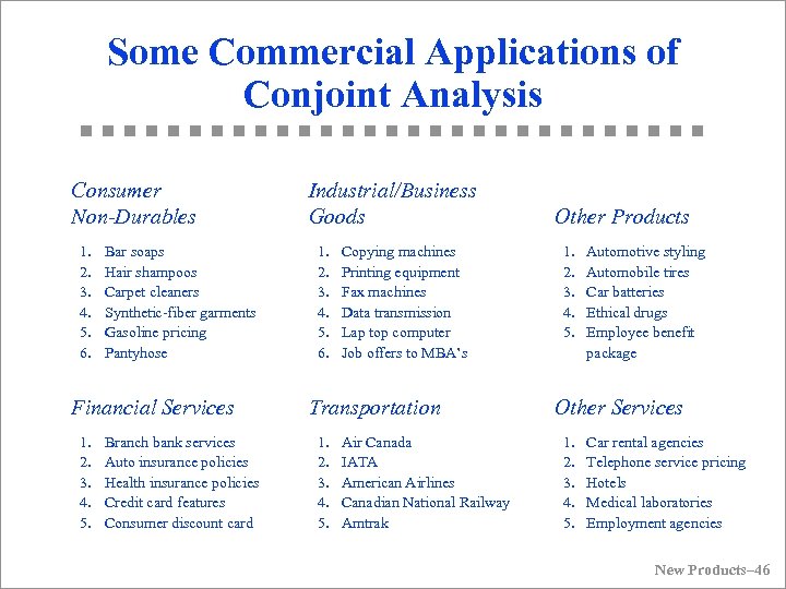Some Commercial Applications of Conjoint Analysis Consumer Non-Durables 1. 2. 3. 4. 5. 6. Bar soaps Hair shampoos Carpet cleaners Synthetic-fiber garments Gasoline pricing Pantyhose Financial Services 1. 2. 3. 4. 5. Branch bank services Auto insurance policies Health insurance policies Credit card features Consumer discount card Industrial/Business Goods 1. 2. 3. 4. 5. 6. Copying machines Printing equipment Fax machines Data transmission Lap top computer Job offers to MBA’s Transportation 1. 2. 3. 4. 5. Air Canada IATA American Airlines Canadian National Railway Amtrak Other Products 1. 2. 3. 4. 5. Automotive styling Automobile tires Car batteries Ethical drugs Employee benefit package Other Services 1. 2. 3. 4. 5. Car rental agencies Telephone service pricing Hotels Medical laboratories Employment agencies New Products– 46

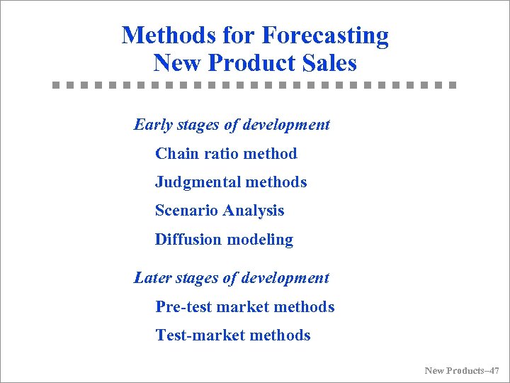Methods for Forecasting New Product Sales Early stages of development Chain ratio method Judgmental methods Scenario Analysis Diffusion modeling Later stages of development Pre-test market methods Test-market methods New Products– 47

The Bass Diffusion Model designed to answer the question: When will customers adopt a new product or technology? New Products– 48

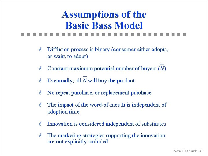Assumptions of the Basic Bass Model G Diffusion process is binary (consumer either adopts, or waits to adopt) G Constant maximum potential number of buyers (N) G Eventually, all N will buy the product G No repeat purchase, or replacement purchase G The impact of the word-of-mouth is independent of adoption time G Innovation is considered independent of substitutes G The marketing strategies supporting the innovation are not explicitly included New Products– 49

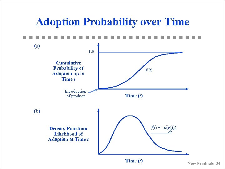Adoption Probability over Time (a) 1. 0 Cumulative Probability of Adoption up to Time t Introduction of product F(t) Time (t) (b) f(t) = d(F(t)) dt Density Function: Likelihood of Adoption at Time (t) New Products– 50

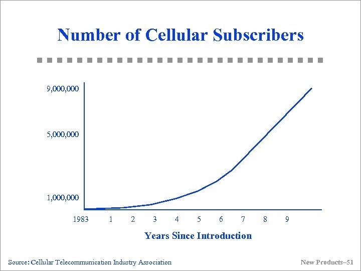Number of Cellular Subscribers 9, 000 5, 000, 000 1983 1 2 3 4 5 6 7 8 9 Years Since Introduction Source: Cellular Telecommunication Industry Association New Products– 51

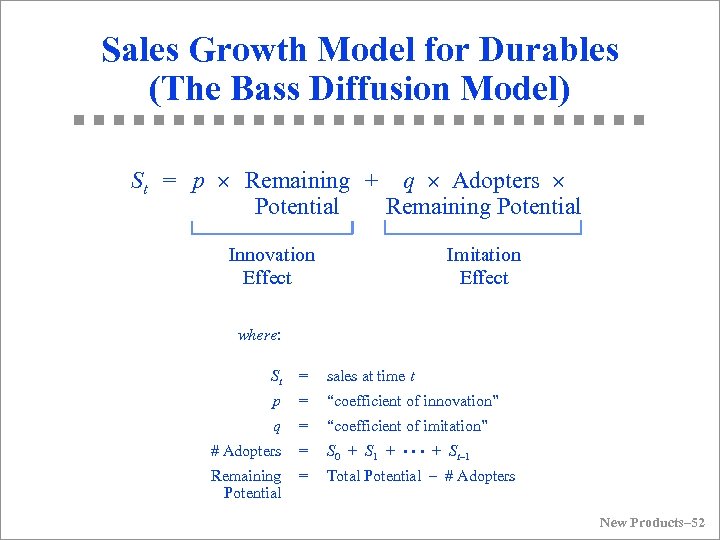Sales Growth Model for Durables (The Bass Diffusion Model) St = p ´ Remaining + q ´ Adopters ´ Potential Remaining Potential Innovation Imitation Effect where: St = sales at time t p = “coefficient of innovation” q = “coefficient of imitation” # Adopters = S 0 + S 1 + • • • + St– 1 Remaining Potential = Total Potential – # Adopters New Products– 52

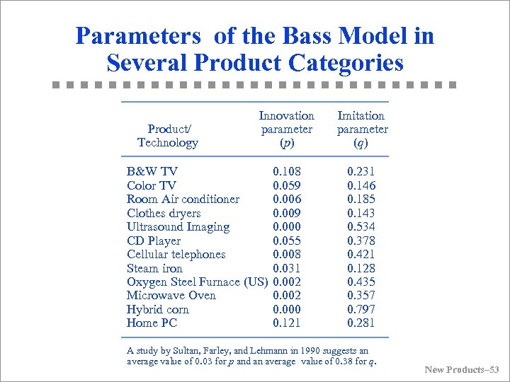Parameters of the Bass Model in Several Product Categories Product/ Technology Innovation parameter (p) B&W TV Color TV Room Air conditioner Clothes dryers Ultrasound Imaging CD Player Cellular telephones Steam iron Oxygen Steel Furnace (US) Microwave Oven Hybrid corn Home PC 0. 108 0. 059 0. 006 0. 009 0. 000 0. 055 0. 008 0. 031 0. 002 0. 000 0. 121 Imitation parameter (q) 0. 231 0. 146 0. 185 0. 143 0. 534 0. 378 0. 421 0. 128 0. 435 0. 357 0. 797 0. 281 A study by Sultan, Farley, and Lehmann in 1990 suggests an average value of 0. 03 for p and an average value of 0. 38 for q. New Products– 53

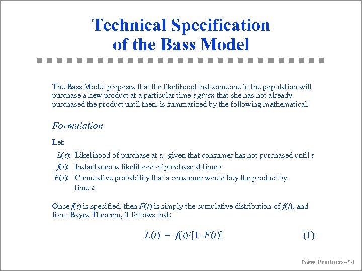Technical Specification of the Bass Model The Bass Model proposes that the likelihood that someone in the population will purchase a new product at a particular time t given that she has not already purchased the product until then, is summarized by the following mathematical. Formulation Let: L(t): Likelihood of purchase at t, given that consumer has not purchased until t f(t): Instantaneous likelihood of purchase at time t F(t): Cumulative probability that a consumer would buy the product by time t Once f(t) is specified, then F(t) is simply the cumulative distribution of f(t), and from Bayes Theorem, it follows that: L(t) = f(t)/[1–F(t)] (1) New Products– 54

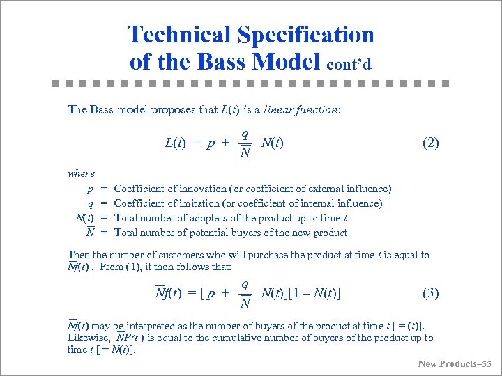Technical Specification of the Bass Model cont’d The Bass model proposes that L(t) is a linear function: q L(t) = p + –– N(t) N where p q N(t) N = = (2) Coefficient of innovation (or coefficient of external influence) Coefficient of imitation (or coefficient of internal influence) Total number of adopters of the product up to time t Total number of potential buyers of the new product Then the number of customers who will purchase the product at time t is equal to Nf(t). From (1), it then follows that: q Nf(t) = [ p + –– N(t)][1 – N(t)] N (3) Nf(t) may be interpreted as the number of buyers of the product at time t [ = (t)]. Likewise, NF(t ) is equal to the cumulative number of buyers of the product up to time t [ = N(t)]. New Products– 55

Bass Model cont’d Noting that [n(t) = Nf(t)] is equal to the number of buyers at time t, and [N(t) = NF(t)] is equal to the cumulative number of buyers until time t, we get from (2): q Nf(t) = [ p + –– N(t)][1 – N(t)] N (3) After simplification, this gives the basic diffusion equation for predicting new product sales: q n (t) = p. N + (q – p) [N(t)] – –– [N(t)]2 N (4) New Products– 56

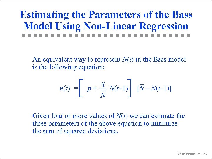Estimating the Parameters of the Bass Model Using Non-Linear Regression An equivalent way to represent N(t) in the Bass model is the following equation: n(t) = q p + –– N(t– 1) [N – N(t– 1)] N Given four or more values of N(t) we can estimate three parameters of the above equation to minimize the sum of squared deviations. New Products– 57

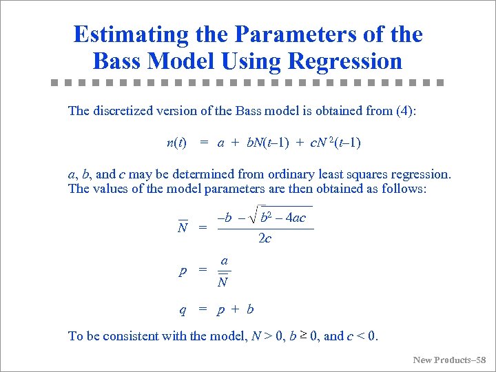Estimating the Parameters of the Bass Model Using Regression The discretized version of the Bass model is obtained from (4): n(t) = a + b. N(t– 1) + c. N 2(t– 1) a, b, and c may be determined from ordinary least squares regression. The values of the model parameters are then obtained as follows: –b – b 2 – 4 ac N = ––––––– 2 c a p = –– N q = p + b To be consistent with the model, N > 0, b 0, and c < 0. New Products– 58

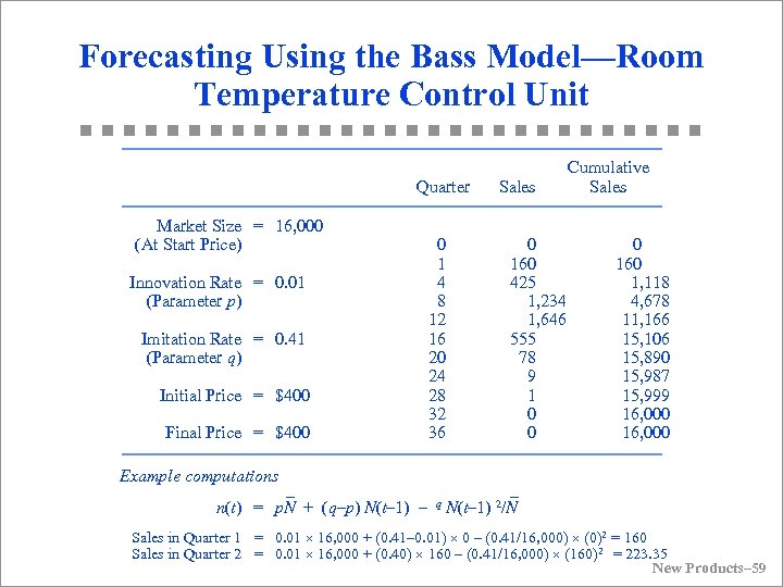Forecasting Using the Bass Model—Room Temperature Control Unit Quarter Market Size = 16, 000 (At Start Price) Innovation Rate = 0. 01 (Parameter p) Imitation Rate = 0. 41 (Parameter q) Initial Price = $400 Final Price = $400 0 1 4 8 12 16 20 24 28 32 36 Sales 0 160 425 1, 234 1, 646 555 78 9 1 0 0 Cumulative Sales 0 160 1, 118 4, 678 11, 166 15, 106 15, 890 15, 987 15, 999 16, 000 Example computations n(t) = p. N + (q–p) N(t– 1) – q N(t– 1) 2/N Sales in Quarter 1 = 0. 01 ´ 16, 000 + (0. 41– 0. 01) ´ 0 – (0. 41/16, 000) ´ (0)2 = 160 Sales in Quarter 2 = 0. 01 ´ 16, 000 + (0. 40) ´ 160 – (0. 41/16, 000) ´ (160)2 = 223. 35 New Products– 59

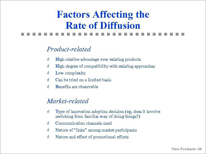Factors Affecting the Rate of Diffusion Product-related G High relative advantage over existing products G High degree of compatibility with existing approaches Low complexity Can be tried on a limited basis Benefits are observable G G G Market-related G G Type of innovation adoption decision (eg, does it involve switching from familiar way of doing things? ) Communication channels used Nature of “links” among market participants Nature and effect of promotional efforts New Products– 60

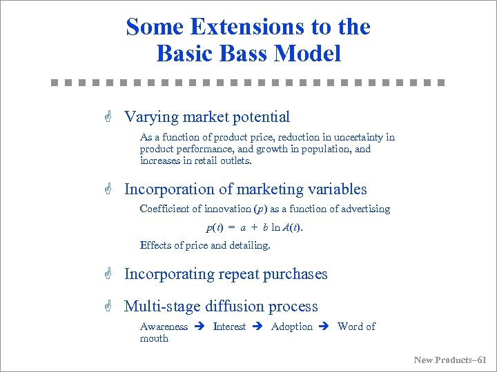Some Extensions to the Basic Bass Model G Varying market potential As a function of product price, reduction in uncertainty in product performance, and growth in population, and increases in retail outlets. G Incorporation of marketing variables Coefficient of innovation (p) as a function of advertising p(t) = a + b ln A(t). Effects of price and detailing. G Incorporating repeat purchases G Multi-stage diffusion process Awareness è Interest è Adoption è Word of mouth New Products– 61

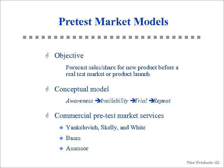Pretest Market Models G Objective Forecast sales/share for new product before a real test market or product launch G Conceptual model Awareness è Availability è Trial è Repeat G Commercial pre-test market services u Yankelovich, Skelly, and White u Bases u Assessor New Products– 62

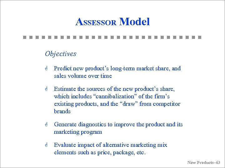ASSESSOR Model Objectives G Predict new product’s long-term market share, and sales volume over time G Estimate the sources of the new product’s share, which includes “cannibalization” of the firm’s existing products, and the “draw” from competitor brands G Generate diagnostics to improve the product and its marketing program G Evaluate impact of alternative marketing mix elements such as price, package, etc. New Products– 63

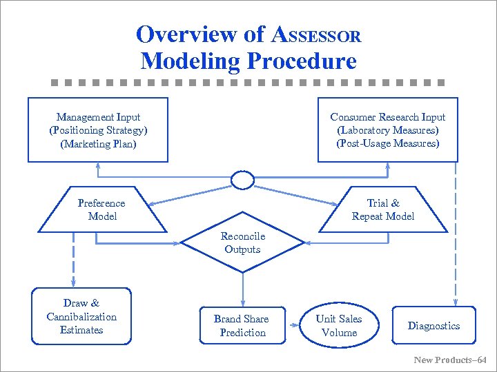Overview of ASSESSOR Modeling Procedure Consumer Research Input (Laboratory Measures) (Post-Usage Measures) Management Input (Positioning Strategy) (Marketing Plan) Preference Model Trial & Repeat Model Reconcile Outputs Draw & Cannibalization Estimates Brand Share Prediction Unit Sales Volume Diagnostics New Products– 64

Overview of ASSESSOR Measurements Design O 1 O 2 X 1 [O 3] X 2 O 4 X 3 O 5 Procedure Respondent screening and recruitment (personal interview) Pre-measurement for established brands (self-administrated questionnaire) Exposure to advertising for established brands and new brands Measurement of reactions to the advertising materials (self administered questionnaire) Simulated shopping trip and exposure to display of new and established brands Purchase opportunity (choice recorded by research personnel) Home use/consumption of new brand Post-usage measurement (telephone Measurement Criteria for target-group identification (eg, product-class usage) Composition of ‘relevant set’ of established brands, attribute weights and ratings, and preferences Optional, e. g. likability and believability ratings of advertising materials Brand(s) purchased New-brand usage rate, satisfaction ratings, and repeat-purchase propensity; attribute ratings and preferences for ‘relevant set’ of established brands plus the new brand O = Measurement; X = Advertsing or product exposure New Products– 65

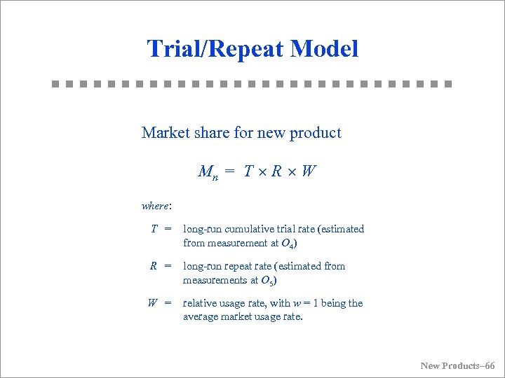Trial/Repeat Model Market share for new product Mn = T ´ R ´ W where: T = long-run cumulative trial rate (estimated from measurement at O 4) R = long-run repeat rate (estimated from measurements at O 5) W = relative usage rate, with w = 1 being the average market usage rate. New Products– 66

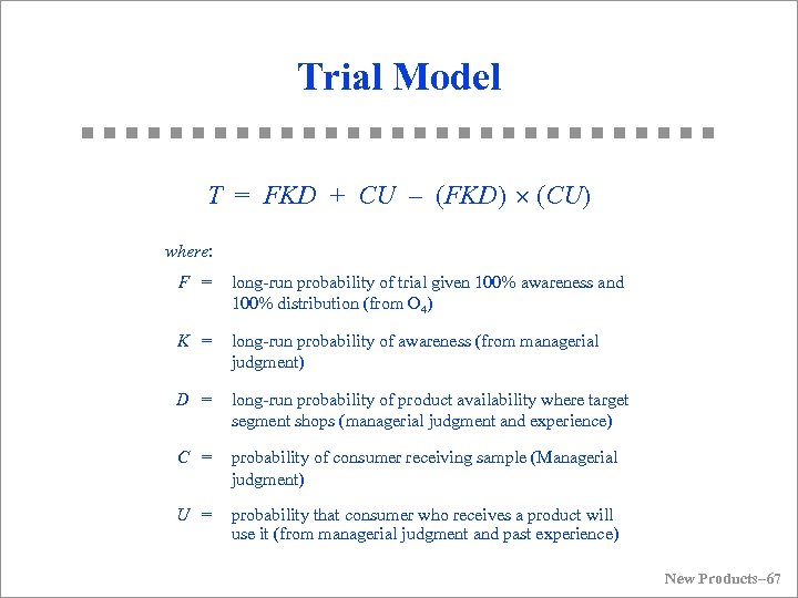Trial Model T = FKD + CU – (FKD) ´ (CU) where: F = long-run probability of trial given 100% awareness and 100% distribution (from O 4) K = long-run probability of awareness (from managerial judgment) D = long-run probability of product availability where target segment shops (managerial judgment and experience) C = probability of consumer receiving sample (Managerial judgment) U = probability that consumer who receives a product will use it (from managerial judgment and past experience) New Products– 67

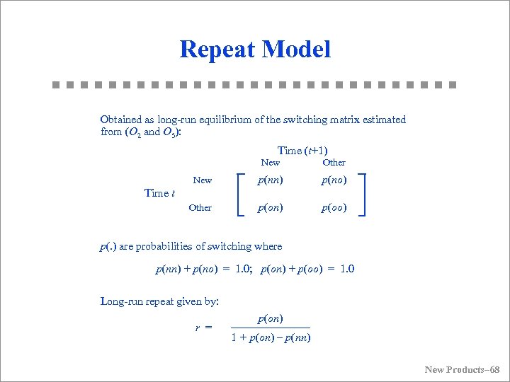Repeat Model Obtained as long-run equilibrium of the switching matrix estimated from (O 2 and O 5): Time (t+1) New Other New p(nn) p(no) Other p(on) p(oo) Time t p(. ) are probabilities of switching where p(nn) + p(no) = 1. 0; p(on) + p(oo) = 1. 0 Long-run repeat given by: r = p(on) ––––––– 1 + p(on) – p(nn) New Products– 68

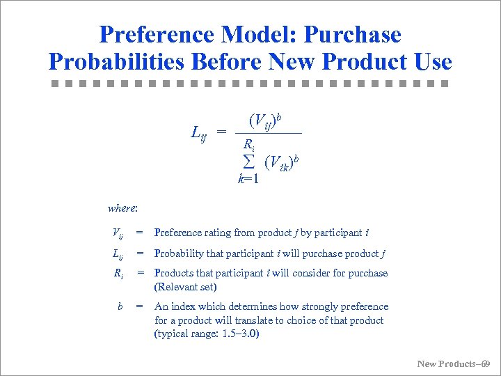Preference Model: Purchase Probabilities Before New Product Use Lij (Vij)b = –––– Ri å (Vik)b k=1 where: Vij = Preference rating from product j by participant i Lij = Probability that participant i will purchase product j Ri = Products that participant i will consider for purchase (Relevant set) b = An index which determines how strongly preference for a product will translate to choice of that product (typical range: 1. 5– 3. 0) New Products– 69

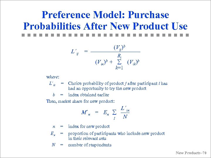Preference Model: Purchase Probabilities After New Product Use L´ij (Vij)b = ––––––––– Ri (Vin)b + å (Vik)b k=1 where: L´it = Choice probability of product j after participant i has had an opportunity to try the new product b = index obtained earlier Then, market share for new product: M´n L´in = En å ––– N I n = index for new product En = N = proportion of participants who include new product in their relevant sets number of respondents New Products– 70

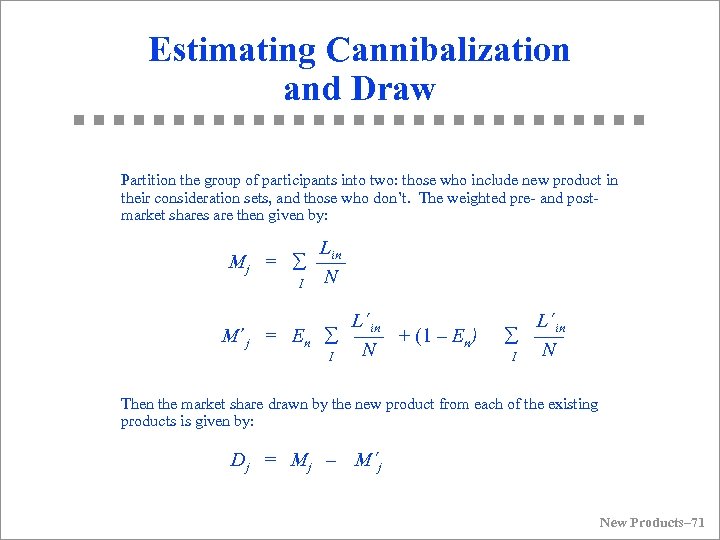Estimating Cannibalization and Draw Partition the group of participants into two: those who include new product in their consideration sets, and those who don’t. The weighted pre- and post- market shares are then given by: Lin Mj = å ––– N I L´in M´j = En å ––– + (1 – En) N I L´in å ––– I N Then the market share drawn by the new product from each of the existing products is given by: Dj = Mj – M´j New Products– 71

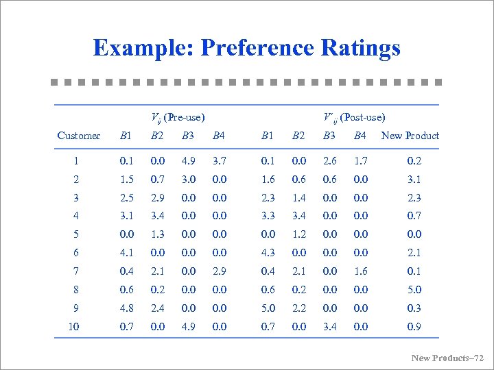Example: Preference Ratings Vij (Pre-use) Customer V´ij (Post-use) B 1 B 2 B 3 B 4 New Product 1 0. 0 4. 9 3. 7 0. 1 0. 0 2. 6 1. 7 0. 2 2 1. 5 0. 7 3. 0 0. 0 1. 6 0. 0 3. 1 3 2. 5 2. 9 0. 0 2. 3 1. 4 0. 0 2. 3 4 3. 1 3. 4 0. 0 3. 3 3. 4 0. 0 0. 7 5 0. 0 1. 3 0. 0 1. 2 0. 0 6 4. 1 0. 0 4. 3 0. 0 2. 1 7 0. 4 2. 1 0. 0 2. 9 0. 4 2. 1 0. 0 1. 6 0. 1 8 0. 6 0. 2 0. 0 5. 0 9 4. 8 2. 4 0. 0 5. 0 2. 2 0. 0 0. 3 10 0. 7 0. 0 4. 9 0. 0 0. 7 0. 0 3. 4 0. 0 0. 9 New Products– 72

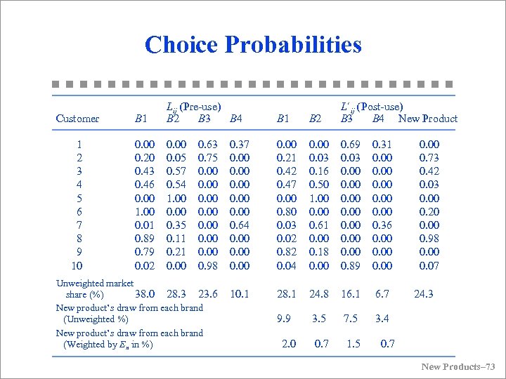Choice Probabilities Customer 1 2 3 4 5 6 7 8 9 10 B 1 Lij (Pre-use) B 2 B 3 B 4 B 1 B 2 L´ij (Post-use) B 3 B 4 New Product 0. 00 0. 20 0. 43 0. 46 0. 00 1. 00 0. 01 0. 89 0. 79 0. 02 0. 00 0. 05 0. 57 0. 54 1. 00 0. 35 0. 11 0. 21 0. 00 0. 37 0. 00 0. 64 0. 00 0. 21 0. 42 0. 47 0. 00 0. 80 0. 03 0. 02 0. 82 0. 04 0. 00 0. 03 0. 16 0. 50 1. 00 0. 61 0. 00 0. 18 0. 00 0. 69 0. 03 0. 00 0. 89 0. 31 0. 00 0. 36 0. 00 10. 1 28. 1 24. 8 16. 1 6. 7 9. 9 3. 5 7. 5 3. 4 2. 0 0. 7 1. 5 0. 7 0. 63 0. 75 0. 00 0. 98 Unweighted market share (%) 38. 0 28. 3 23. 6 New product’s draw from each brand (Unweighted %) New product’s draw from each brand (Weighted by En in %) 0. 00 0. 73 0. 42 0. 03 0. 00 0. 20 0. 00 0. 98 0. 00 0. 07 24. 3 New Products– 73

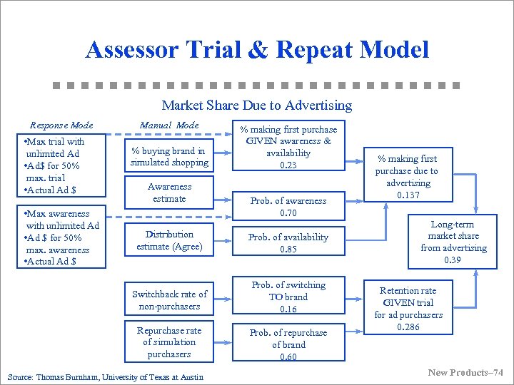Assessor Trial & Repeat Model Market Share Due to Advertising Response Mode • Max trial with unlimited Ad • Ad$ for 50% max. trial • Actual Ad $ • Max awareness with unlimited Ad • Ad $ for 50% max. awareness • Actual Ad $ Manual Mode % buying brand in simulated shopping Awareness estimate % making first purchase GIVEN awareness & availability 0. 23 Prob. of awareness 0. 70 Distribution estimate (Agree) Prob. of availability 0. 85 Switchback rate of non-purchasers Prob. of switching TO brand 0. 16 Repurchase rate of simulation purchasers Prob. of repurchase of brand 0. 60 Source: Thomas Burnham, University of Texas at Austin % making first purchase due to advertising 0. 137 Long-term market share from advertising 0. 39 Retention rate GIVEN trial for ad purchasers 0. 286 New Products– 74

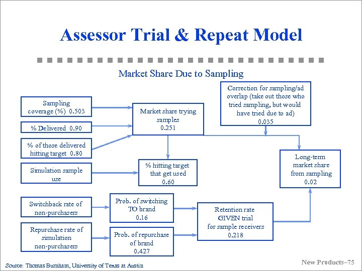Assessor Trial & Repeat Model Market Share Due to Sampling coverage (%) 0. 503 % Delivered 0. 90 Market share trying samples 0. 251 Correction for sampling/ad overlap (take out those who tried sampling, but would have tried due to ad) 0. 035 % of those delivered hitting target 0. 80 % hitting target that get used 0. 60 Simulation sample use Switchback rate of non-purchasers Repurchase rate of simulation non-purchasers Long-term market share from sampling 0. 02 Prob. of switching TO brand 0. 16 Prob. of repurchase of brand 0. 427 Source: Thomas Burnham, University of Texas at Austin Retention rate GIVEN trial for sample receivers 0. 218 New Products– 75

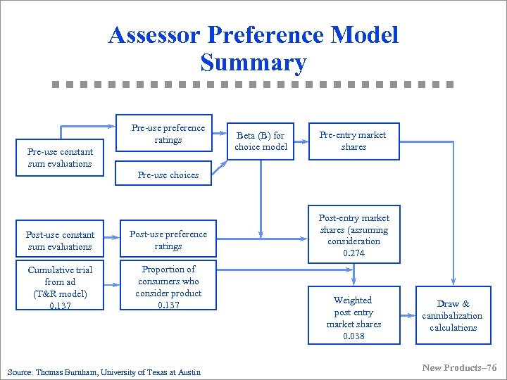Assessor Preference Model Summary Pre-use preference ratings Pre-use constant sum evaluations Beta (B) for choice model Pre-entry market shares Pre-use choices Post-use constant sum evaluations Post-use preference ratings Cumulative trial from ad (T&R model) 0. 137 Proportion of consumers who consider product 0. 137 Source: Thomas Burnham, University of Texas at Austin Post-entry market shares (assuming consideration 0. 274 Weighted post entry market shares 0. 038 Draw & cannibalization calculations New Products– 76

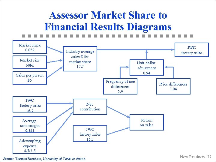Assessor Market Share to Financial Results Diagrams Market share 0. 059 Market size 60 M Industry average sales $ for market share 17. 7 Sales person $5 JWC factory sales 16. 7 Average unit margin 0. 541 Ad/sampling expense 4. 5/3. 5 JWC factory sales Unit-dollar adjustment 0. 94 Frequency of use differences 0. 9 Price differences 1. 04 Net contribution JWC factory sales 16. 7 Source: Thomas Burnham, University of Texas at Austin Return on sales New Products– 77

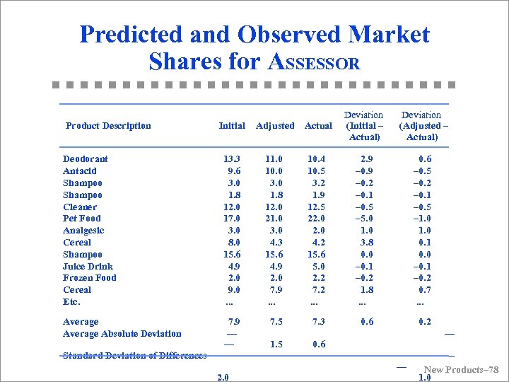Predicted and Observed Market Shares for ASSESSOR Product Description Deviation Initial Adjusted Actual (Initial – Actual) Deviation (Adjusted – Actual) Deodorant Antacid Shampoo Cleaner Pet Food Analgesic Cereal Shampoo Juice Drink Frozen Food Cereal Etc. 13. 3 9. 6 3. 0 1. 8 12. 0 17. 0 3. 0 8. 0 15. 6 4. 9 2. 0 9. 0 . . . 2. 9 – 0. 2 – 0. 1 – 0. 5 – 5. 0 1. 0 3. 8 0. 0 – 0. 1 – 0. 2 1. 8. . . 0. 6 Average Absolute Deviation 7. 9 — — Standard Deviation of Differences — 2. 0 11. 0 10. 0 3. 0 1. 8 12. 0 21. 0 3. 0 4. 3 15. 6 4. 9 2. 0 7. 9. . . 10. 4 10. 5 3. 2 1. 9 12. 5 22. 0 4. 2 15. 6 5. 0 2. 2 7. 2 . . . 7. 5 7. 3 1. 5 0. 6 0. 6 – 0. 5 – 0. 2 – 0. 1 – 0. 5 – 1. 0 0. 1 0. 0 – 0. 1 – 0. 2 0. 7 . . . 0. 2 — — — New Products– 78 1. 0

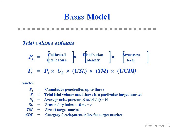BASES Model Trial volume estimate Pt = Calibrated intent score Distribution intensityt Awareness levelt Tt = Pt U 0 (1/Sit) (TM) (1/CDI) where: Pt Tt U 0 Sit TM CDI = = = Cumulative penetration up to time t Total trial volume until time t in a particular target market Average units purchased at trial (t = 0) Seasonality index at time = t Size of target market Category development index for target market New Products– 79

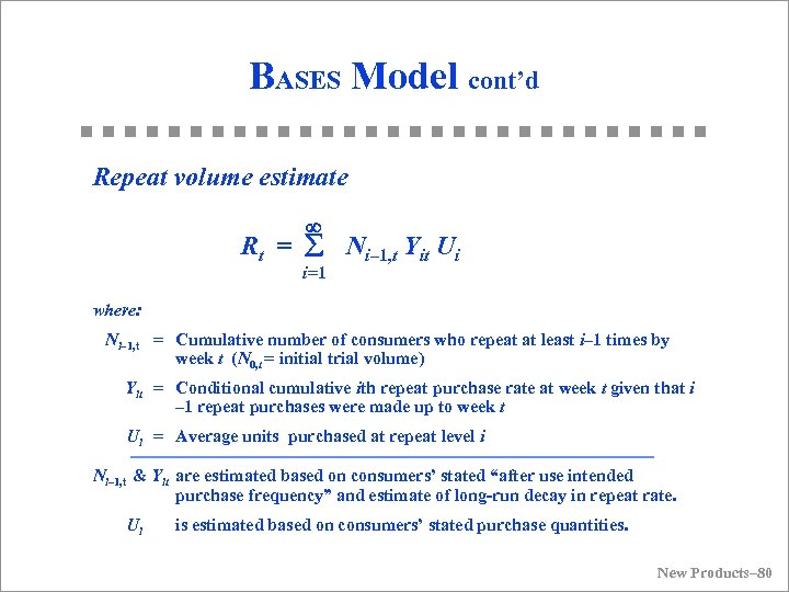BASES Model cont’d Repeat volume estimate ¥ Rt = å Ni– 1, t Yit Ui i=1 where: Ni– 1, t = Cumulative number of consumers who repeat at least i– 1 times by week t (N 0, t = initial trial volume) Yit = Conditional cumulative ith repeat purchase rate at week t given that i – 1 repeat purchases were made up to week t Ui = Average units purchased at repeat level i Ni– 1, t & Yit are estimated based on consumers’ stated “after use intended purchase frequency” and estimate of long-run decay in repeat rate. Ui is estimated based on consumers’ stated purchase quantities. New Products– 80

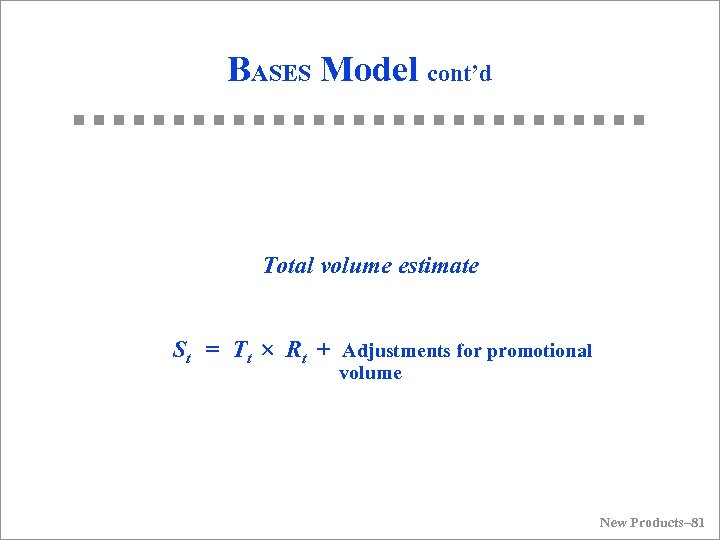BASES Model cont’d Total volume estimate St = Tt Rt + Adjustments for promotional volume New Products– 81

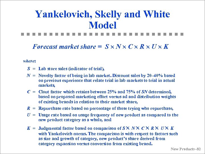Yankelovich, Skelly and White Model Forecast market share = S N C R U K where: S = Lab store sales (indicator of trial), N = Novelty factor of being in lab market. Discount sales by 20– 40% based on previous experience that relate trial in lab markets to trial in actual markets, C = Clout factor which retains between 25% and 75% of SN determined, based on proposed marketing effort versus ad and distribution weights of existing brands in relation to their market share, R = Repurchase rate based on percentage of those trying who repurchase, U = Usage rate based on usage frequency of new product as compared to the new product category as a whole, and K = Judgmental factor based on comparison of S N C R U K with Yankelovich norms. The comparison is with respect to factors such as size and growth of category, new product’s share derived from category expansion versus conversion from existing brand. New Products– 82

Some Issues in Validating Pre-Test Models G Validation does not include products that were withdrawn as a result of model predictions G Pre-test and actual launch are separated in time, often by a year or more G Marketing program as implemented could be different from planned program New Products– 83