Natural Forecasting Asset Pricing and Macroeconomic Dynamics Andreas

Natural Forecasting, Asset Pricing, and Macroeconomic Dynamics Andreas Fuster David Laibson Brock Mendel Harvard University May 2010

Financial crises Key ingredients (Kindleberger 1978) • Improving fundamentals • Rising asset prices • Rising leverage supporting consumption and investment • Falling asset prices and deleveraging • Banking crisis • Recession/Depression

Financial crises Key ingredients (Kindleberger 1978) • Improving fundamentals • Rising asset prices (“bubble”) • Rising leverage supporting consumption and investment • Falling asset prices and deleveraging • Banking crisis • Recession/Depression

Bubbles • Neo-classical economic view: – Non-rational bubbles don’t exist – Non-rational bubbles only appear to exist because of hindsight bias (fundamentals sometimes unexpectedly deteriorate) – Rational bubbles may exist in special circumstances (Tirole, 1985) • Today: – bubbles are (at least partially) not rational – bubbles explain macro dynamics

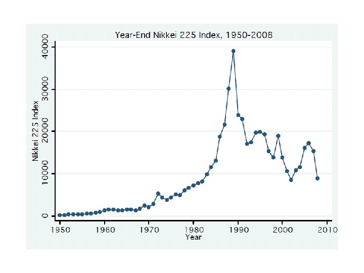
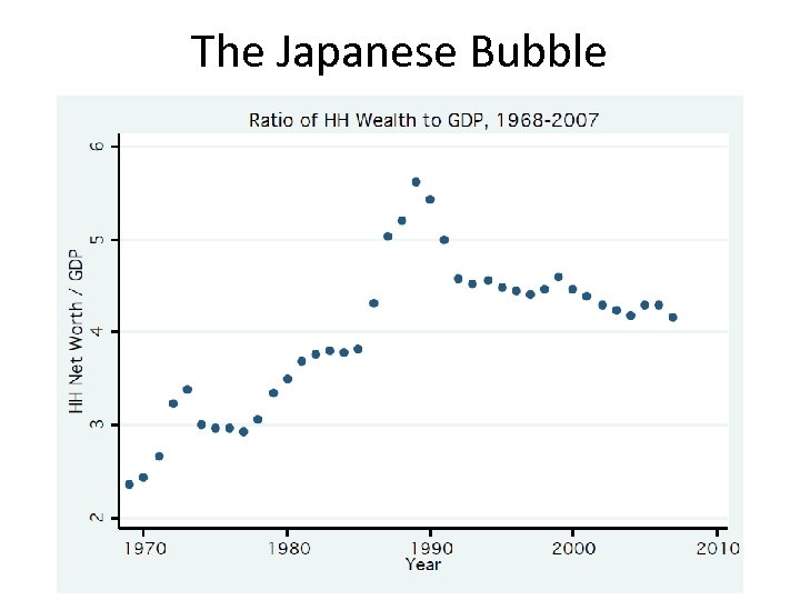The Japanese Bubble

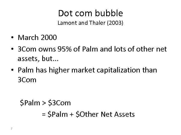Dot com bubble Lamont and Thaler (2003) • March 2000 • 3 Com owns 95% of Palm and lots of other net assets, but. . . • Palm has higher market capitalization than 3 Com $Palm > $3 Com = $Palm + $Other Net Assets 7

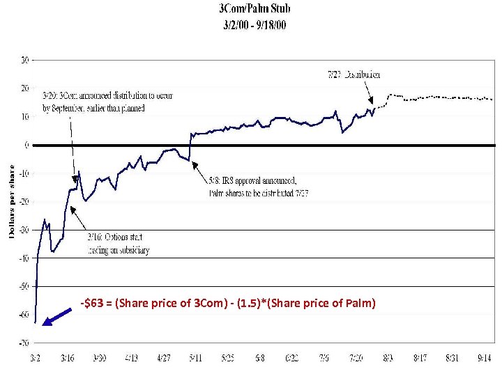-$63 = (Share price of 3 Com) - (1. 5)*(Share price of Palm) 8

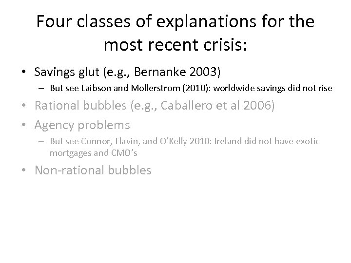Four classes of explanations for the most recent crisis: • Savings glut (e. g. , Bernanke 2003) – But see Laibson and Mollerstrom (2010): worldwide savings did not rise • Rational bubbles (e. g. , Caballero et al 2006) • Agency problems – But see Connor, Flavin, and O’Kelly 2010: Ireland did not have exotic mortgages and CMO’s • Non-rational bubbles

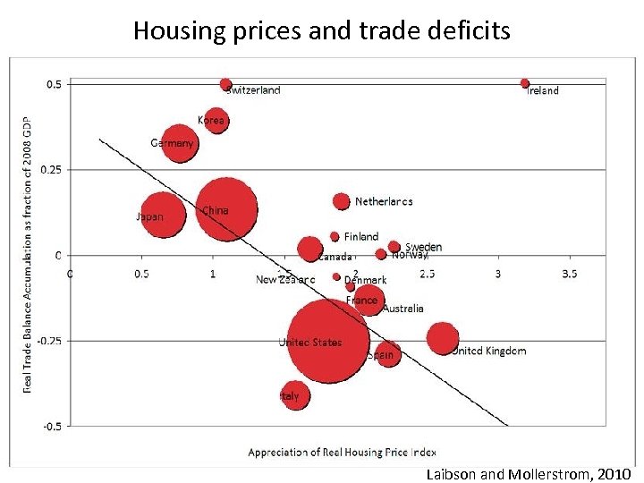Housing prices and trade deficits Germany Japan Turkey Laibson and Mollerstrom, 2010

Four classes of explanations for the most recent crisis: • Savings glut (e. g. , Bernanke 2003) – But see Laibson and Mollerstrom (2010): worldwide savings did not rise • Rational bubbles (e. g. , Caballero et al 2006) • Agency problems – But see Connor, Flavin, and O’Kelly 2010: Ireland did not have exotic mortgages and CMO’s • Non-rational bubbles

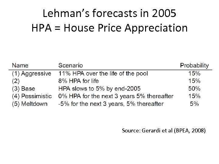Lehman’s forecasts in 2005 HPA = House Price Appreciation Source: Gerardi et al (BPEA, 2008)

Alan Greenspan • “While local economies may experience significant speculative price imbalances, a national severe price distortion seems most unlikely in the United States, given its size and diversity. ” (October, 2004) • If home prices do decline, that “likely would not have substantial macroeconomic implications. ” (June, 2005) • Though housing prices are likely to be lower than the year before, “I think the worst of this may well be over. ” (October, 2006)

Four classes of explanations for the most recent crisis: • Savings glut (e. g. , Bernanke 2003) – But see Laibson and Mollerstrom (2010): worldwide savings did not rise • Rational bubbles (e. g. , Caballero et al 2006) • Agency problems – But see Connor, Flavin, and O’Kelly 2010: Ireland did not have exotic mortgages and CMO’s • Non-rational bubbles

Bubbles form: 1995 -2007 • I’ll focus on the US • Related bubbles existed in many other countries • The US bubble had two main components: – Prices of publicly traded companies – Prices of residential real estate • And many minor contributors: – Prices of private equity – Commodities – Hedge funds

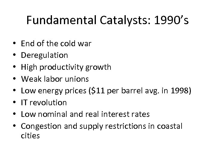Fundamental Catalysts: 1990’s • • End of the cold war Deregulation High productivity growth Weak labor unions Low energy prices ($11 per barrel avg. in 1998) IT revolution Low nominal and real interest rates Congestion and supply restrictions in coastal cities

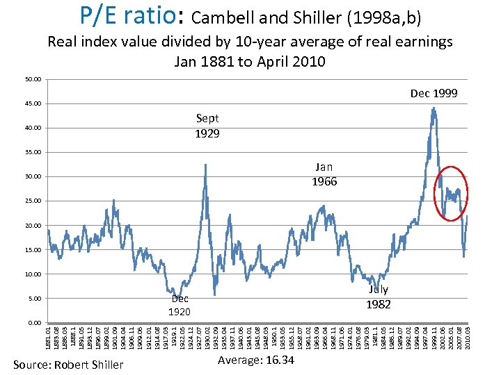1881. 01 1883. 08 1886. 03 1888. 1 1891. 05 1893. 12 1896. 07 1899. 02 1901. 09 1904. 04 1906. 11 1909. 06 1912. 01 1914. 08 1917. 03 1919. 1 1922. 05 1924. 12 1927. 07 1930. 02 1932. 09 1935. 04 1937. 11 1940. 06 1943. 01 1945. 08 1948. 03 1950. 1 1953. 05 1955. 12 1958. 07 1961. 02 1963. 09 1966. 04 1968. 11 1971. 06 1974. 01 1976. 08 1979. 03 1981. 1 1984. 05 1986. 12 1989. 07 1992. 02 1994. 09 1997. 04 1999. 11 2002. 06 2005. 01 2007. 08 2010. 03 P/E ratio: Cambell and Shiller (1998 a, b) Real index value divided by 10 -year average of real earnings Jan 1881 to April 2010 50. 00 45. 00 Dec 1999 40. 00 Sept 1929 35. 00 30. 00 Jan 1966 25. 00 20. 00 15. 00 10. 00 5. 00 Dec 1920 Source: Robert Shiller July 1982 0. 00 Average: 16. 34

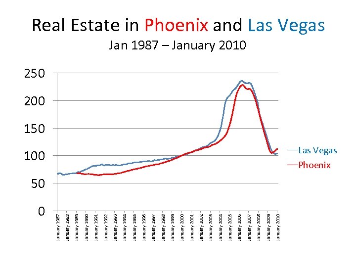0 January 2010 January 2009 January 2008 January 2007 January 2006 January 2005 January 2004 January 2003 January 2002 January 2001 January 2000 January 1999 January 1998 January 1997 January 1996 January 1995 January 1994 January 1993 January 1992 January 1991 January 1990 January 1989 January 1988 January 1987 Real Estate in Phoenix and Las Vegas Jan 1987 – January 2010 250 200 150 100 Las Vegas Phoenix 50

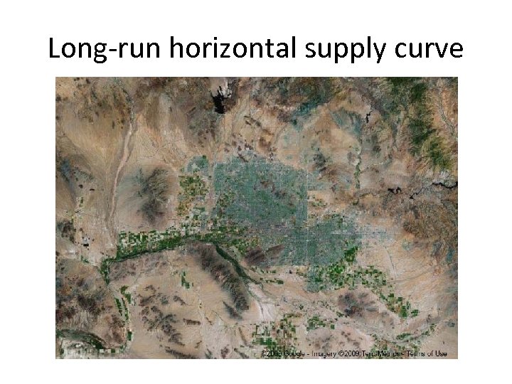Long-run horizontal supply curve Phoenix

Long-run horizontal supply curve Phoenix

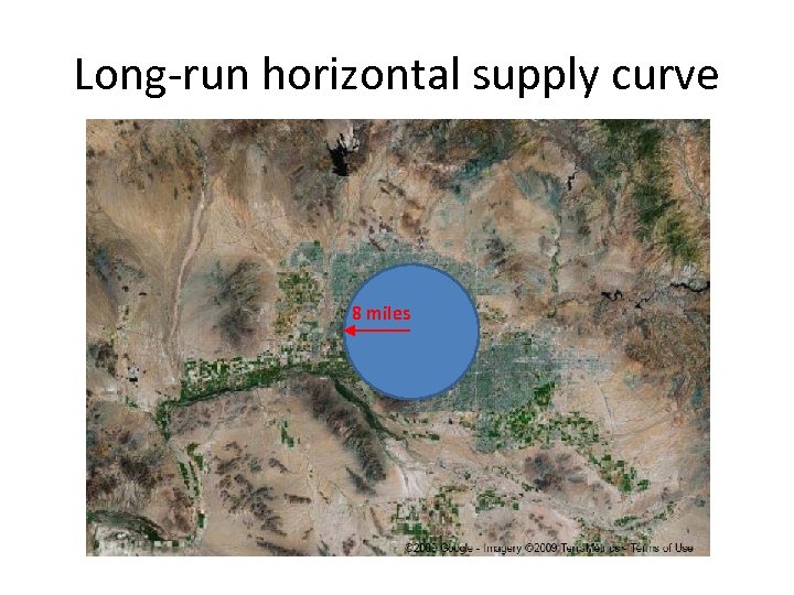Long-run horizontal supply curve 8 miles

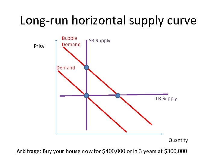Long-run horizontal supply curve Price Bubble Demand SR Supply Demand LR Supply Quantity Arbitrage: Buy your house now for $400, 000 or in 3 years at $300, 000

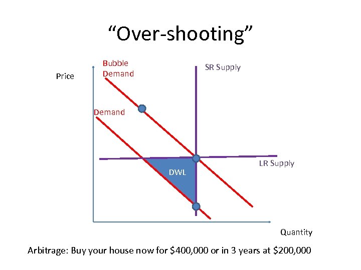“Over-shooting” Price Bubble Demand SR Supply Demand DWL LR Supply Quantity Arbitrage: Buy your house now for $400, 000 or in 3 years at $200, 000

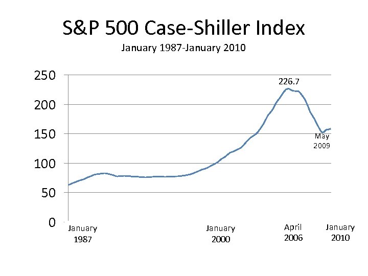0 1 7 13 19 25 31 37 43 49 55 61 67 73 79 85 91 97 103 109 115 121 127 133 139 145 151 157 163 169 175 181 187 193 199 205 211 217 223 229 235 241 247 253 259 265 271 277 S&P 500 Case-Shiller Index January 1987 -January 2010 250 226. 7 200 150 May 2009 100 50 January 1987 January 2000 April 2006 January 2010

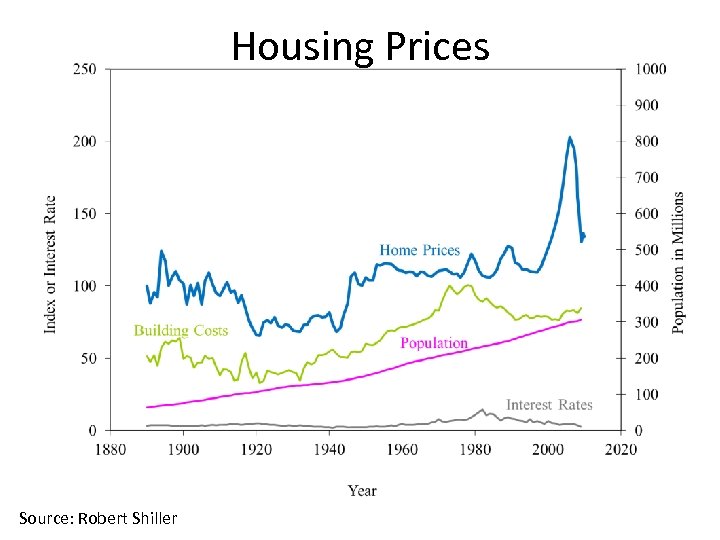Housing Prices Source: Robert Shiller

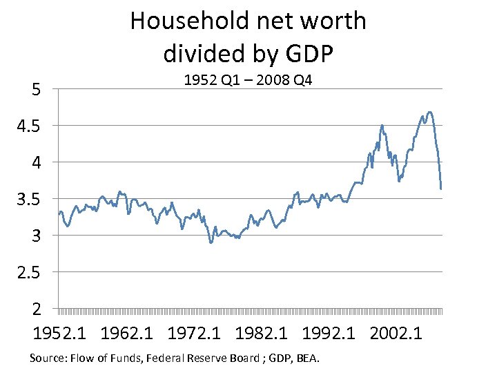Household net worth divided by GDP 5 1952 Q 1 – 2008 Q 4 4. 5 4 3. 5 3 2. 5 2 1952. 1 1962. 1 1972. 1 1982. 1 1992. 1 2002. 1 Source: Flow of Funds, Federal Reserve Board ; GDP, BEA.

Today • • A formal model of non-rational bubbles Microfoundations Testable predictions Goal: Study non-rational expectations with a parsimonious and generalizable model.

Outline 1. Two building blocks – Natural forecasting – Hump-shaped impulse response 2. 3. 4. 5. Tree model Simulations, predictions, empirical evaluation Counterfactuals Extensions

Related Literature • • • • • • Barberis, Shleifer, and Vishny (1998): extrapolative dividend forecasts Barsky and De Long (1993): extrapolation and excess volatility Benartzi (2001): extrapolation and company stock Black (1986): noise traders Campbell and Shiller (1988 a, b): P/E ratio and return predictability Choi (2006): extrapolation and asset pricing Choi, Laibson, and Madrian (2009): positive feedback in investment Cutler, Poterba, and Summers (1991): return autocorrelations De Long, et al (1990): noise traders and positive feedback Hong and Stein (1999): forecasting biases Keynes (1936): animal spirits La. Porta (1996): Growth expectations have insufficient mean reversion Leroy and Porter (1981): excess volatility in stock prices Lettau and Ludvigson (1991): W/C correlates negatively with future returns Lo and Mac. Kinlay (1988): variance ratio tests Loewenstein, O’Donoghue, and Rabin (2003): projection bias Piazessi and Schneider (2009): extrapolative beliefs in the housing market Previterro (2001): extrapolative beliefs and annuity investment Shiller (1981): excess volatility in stock prices Summers (1986): power problems in financial econometrics Tortorice (2010): extrapolative beliefs in unemployment forecasts

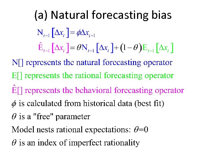(a) Natural forecasting bias

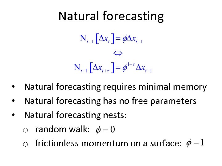Natural forecasting • Natural forecasting requires minimal memory • Natural forecasting has no free parameters • Natural forecasting nests: o random walk: o frictionless momentum on a surface:

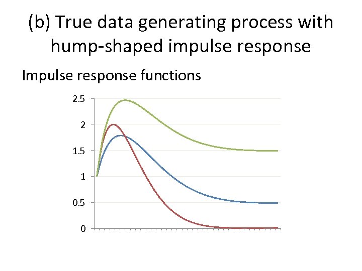(b) True data generating process with hump-shaped impulse response Impulse response functions 2. 5 2 1. 5 1 0. 5 0 1 2 3 4 5 6 7 8 9 101112131415161718192021222324252627282930313233343536

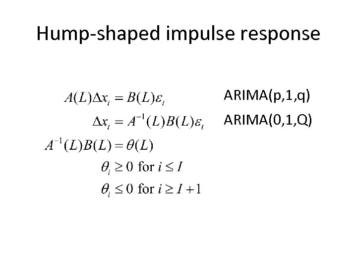Hump-shaped impulse response ARIMA(p, 1, q) ARIMA(0, 1, Q)

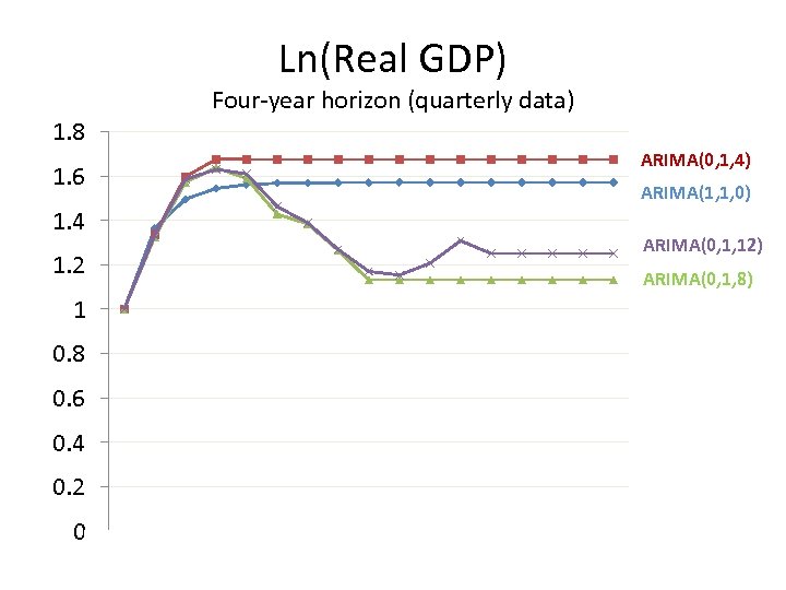Ln(Real GDP) Four-year horizon (quarterly data) 1. 8 ARIMA(0, 1, 4) 1. 6 ARIMA(1, 1, 0) 1. 4 ARIMA(0, 1, 12) 1. 2 ARIMA(0, 1, 8) 1 0. 8 0. 6 0. 4 0. 2 0 0 1 2 3 4 Arima(1, 1, 0) 5 6 7 Arima(0, 1, 4) 8 9 Arima(0, 1, 8) 10 11 12 Arima(0, 1, 12) 13 14 15 16

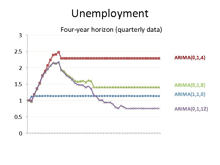Unemployment 3 Four-year horizon (quarterly data) 2. 5 ARIMA(0, 1, 4) 2 1. 5 ARIMA(0, 1, 8) ARIMA(1, 1, 0) 1 ARIMA(0, 1, 12) 0. 5 0 1 2 3 4 5 6 7 8 9 10111213141516171819202122232425262728293031323334353637383940414243444546474849 Arima(1, 1, 0) Arima(0, 1, 12) Arima(0, 1, 24) Arima(0, 1, 36)

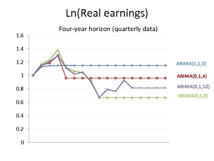Ln(Real earnings) Four-year horizon (quarterly data) 1. 6 1. 4 1. 2 ARIMA(1, 1, 0) 1 ARIMA(0, 1, 4) ARIMA(0, 1, 12) 0. 8 ARIMA(0, 1, 8) 0. 6 0. 4 0. 2 0 0 1 2 3 4 Arima(1, 1, 0) 5 6 7 Arima(0, 1, 4) 8 9 10 Arima(0, 1, 8) 11 12 13 Arima(0, 1, 12) 14 15 16

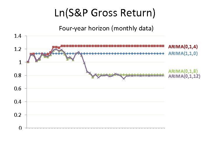Ln(S&P Gross Return) Four-year horizon (monthly data) 1. 4 ARIMA(0, 1, 4) ARIMA(1, 1, 0) 1. 2 1 ARIMA(0, 1, 8) ARIMA(0, 1, 12) 0. 8 0. 6 0. 4 0. 2 0 0 1 2 3 4 5 6 7 8 9 10 11 12 13 14 15 16 17 18 19 20 21 22 23 24 25 26 27 28 29 30 31 32 33 34 35 36 37 38 39 40 41 42 43 44 45 46 47 48 Arima(1, 1, 0) Arima(0, 1, 12) Arima(0, 1, 24) Arima(0, 1, 36)

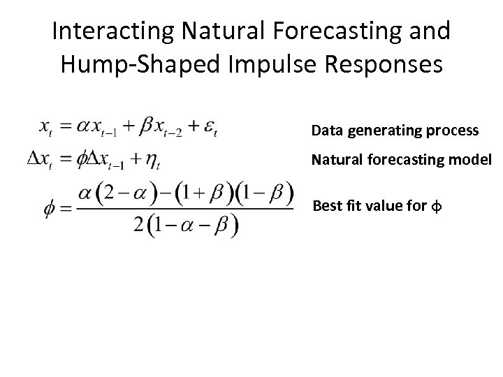Interacting Natural Forecasting and Hump-Shaped Impulse Responses Data generating process Natural forecasting model Best fit value for φ

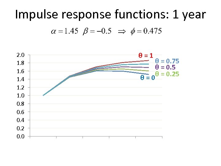Impulse response functions: 1 year θ=1 2. 0 1. 8 1. 6 1. 4 1. 2 1. 0 0. 8 0. 6 0. 4 0. 2 0. 0 θ = 0. 75 θ = 0. 25 θ=0 1 2 3 4 5

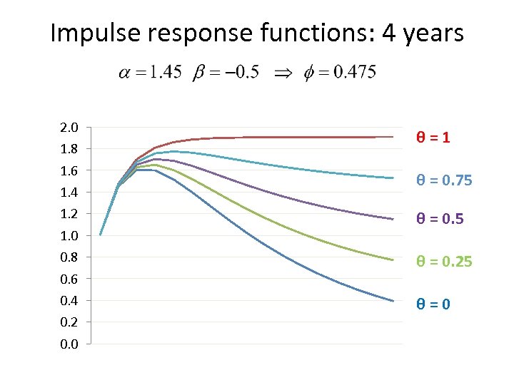Impulse response functions: 4 years 2. 0 1. 8 1. 6 1. 4 1. 2 1. 0 0. 8 0. 6 0. 4 0. 2 0. 0 θ=1 θ = 0. 75 θ = 0. 25 θ=0

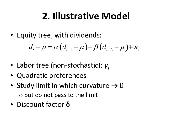2. Illustrative Model • Equity tree, with dividends: • Labor tree (non-stochastic): yt • Quadratic preferences • Study limit in which curvature → 0 o but do not pass to the limit • Discount factor δ

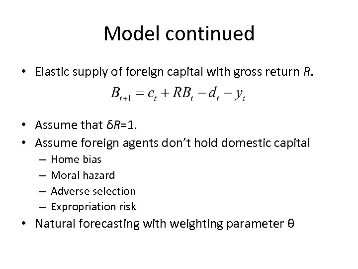Model continued • Elastic supply of foreign capital with gross return R. • Assume that δR=1. • Assume foreign agents don’t hold domestic capital – – Home bias Moral hazard Adverse selection Expropriation risk • Natural forecasting with weighting parameter θ

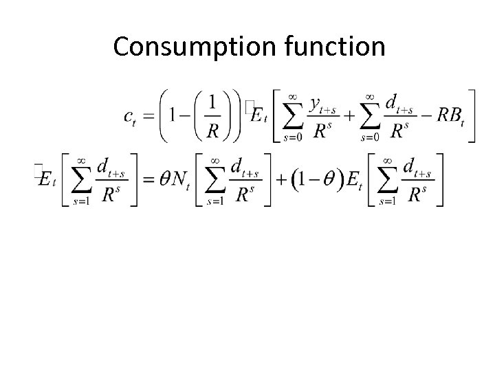Consumption function

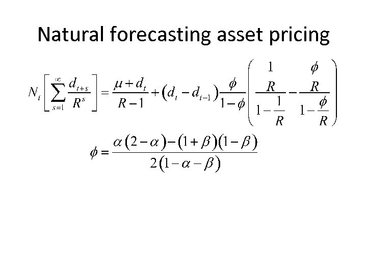Natural forecasting asset pricing

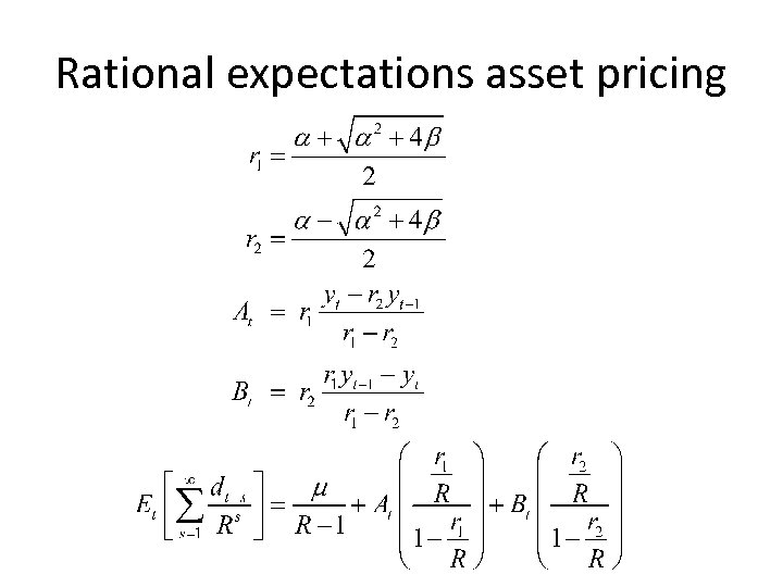Rational expectations asset pricing

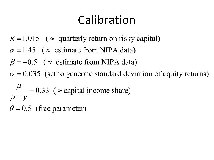Calibration

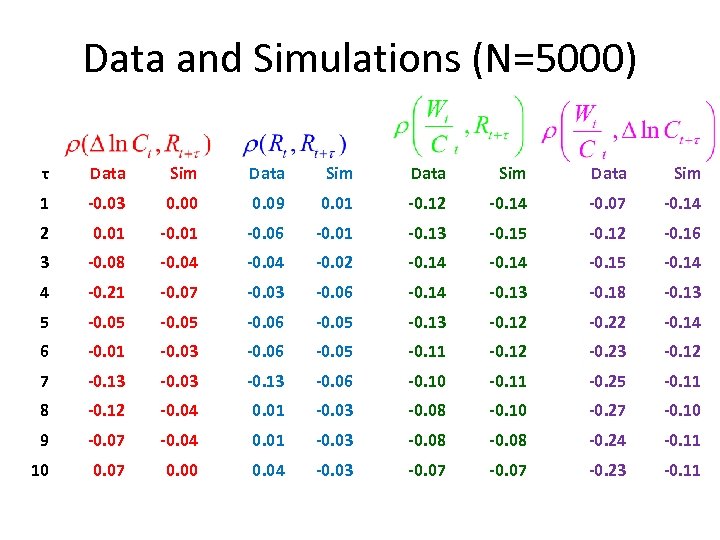Data and Simulations (N=5000) τ Data Sim 1 -0. 03 0. 00 0. 09 0. 01 -0. 12 -0. 14 -0. 07 -0. 14 2 0. 01 -0. 06 -0. 01 -0. 13 -0. 15 -0. 12 -0. 16 3 -0. 08 -0. 04 -0. 02 -0. 14 -0. 15 -0. 14 4 -0. 21 -0. 07 -0. 03 -0. 06 -0. 14 -0. 13 -0. 18 -0. 13 5 -0. 05 -0. 06 -0. 05 -0. 13 -0. 12 -0. 22 -0. 14 6 -0. 01 -0. 03 -0. 06 -0. 05 -0. 11 -0. 12 -0. 23 -0. 12 7 -0. 13 -0. 03 -0. 13 -0. 06 -0. 10 -0. 11 -0. 25 -0. 11 8 -0. 12 -0. 04 0. 01 -0. 03 -0. 08 -0. 10 -0. 27 -0. 10 9 -0. 07 -0. 04 0. 01 -0. 03 -0. 08 -0. 24 -0. 11 10 0. 07 0. 00 0. 04 -0. 03 -0. 07 -0. 23 -0. 11

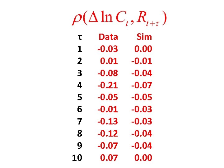τ 1 2 3 4 5 6 7 8 9 10 Data -0. 03 0. 01 -0. 08 -0. 21 -0. 05 -0. 01 -0. 13 -0. 12 -0. 07 Sim 0. 00 -0. 01 -0. 04 -0. 07 -0. 05 -0. 03 -0. 04 0. 00

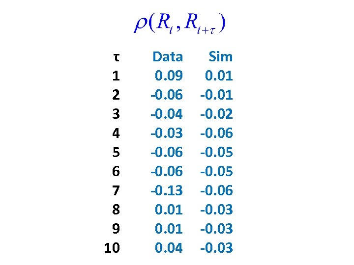τ 1 2 3 4 5 6 7 8 9 10 Data 0. 09 -0. 06 -0. 04 -0. 03 -0. 06 -0. 13 0. 01 0. 04 Sim 0. 01 -0. 02 -0. 06 -0. 05 -0. 06 -0. 03

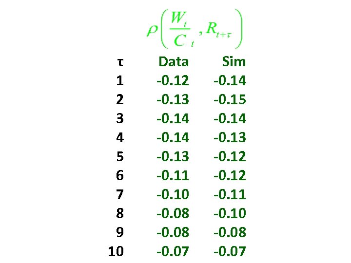τ 1 2 3 4 5 6 7 8 9 10 Data -0. 12 -0. 13 -0. 14 -0. 13 -0. 11 -0. 10 -0. 08 -0. 07 Sim -0. 14 -0. 15 -0. 14 -0. 13 -0. 12 -0. 11 -0. 10 -0. 08 -0. 07

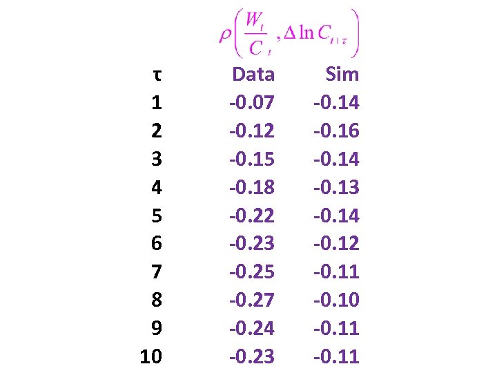τ 1 2 3 4 5 6 7 8 9 10 Data -0. 07 -0. 12 -0. 15 -0. 18 -0. 22 -0. 23 -0. 25 -0. 27 -0. 24 -0. 23 Sim -0. 14 -0. 16 -0. 14 -0. 13 -0. 14 -0. 12 -0. 11 -0. 10 -0. 11

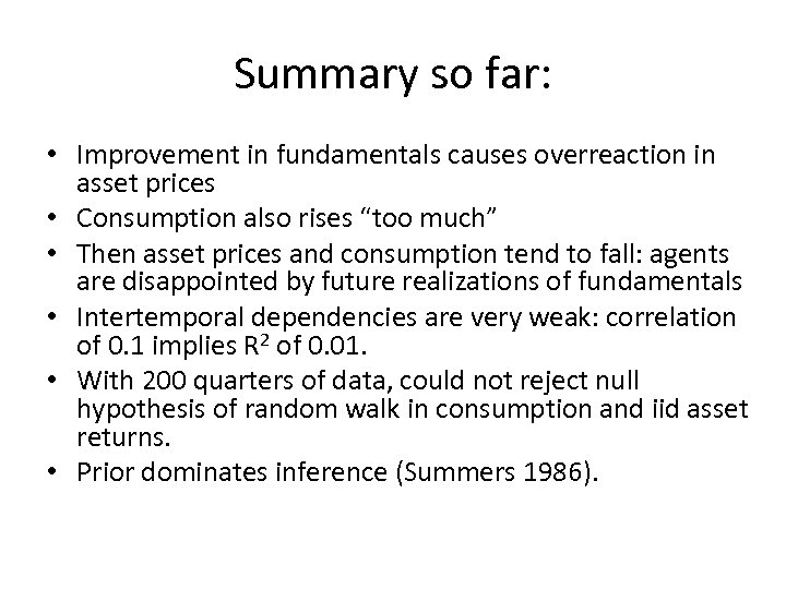Summary so far: • Improvement in fundamentals causes overreaction in asset prices • Consumption also rises “too much” • Then asset prices and consumption tend to fall: agents are disappointed by future realizations of fundamentals • Intertemporal dependencies are very weak: correlation of 0. 1 implies R 2 of 0. 01. • With 200 quarters of data, could not reject null hypothesis of random walk in consumption and iid asset returns. • Prior dominates inference (Summers 1986).

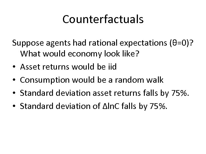Counterfactuals Suppose agents had rational expectations (θ=0)? What would economy look like? • Asset returns would be iid • Consumption would be a random walk • Standard deviation asset returns falls by 75%. • Standard deviation of Δln. C falls by 75%.

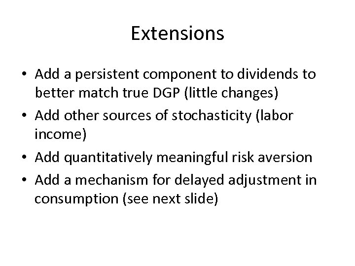Extensions • Add a persistent component to dividends to better match true DGP (little changes) • Add other sources of stochasticity (labor income) • Add quantitatively meaningful risk aversion • Add a mechanism for delayed adjustment in consumption (see next slide)

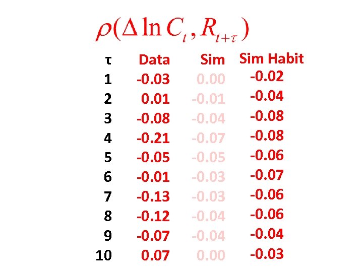τ 1 2 3 4 5 6 7 8 9 10 Data -0. 03 0. 01 -0. 08 -0. 21 -0. 05 -0. 01 -0. 13 -0. 12 -0. 07 Sim Habit -0. 02 0. 00 -0. 04 -0. 01 -0. 08 -0. 04 -0. 08 -0. 07 -0. 06 -0. 05 -0. 07 -0. 03 -0. 06 -0. 04 -0. 03 0. 00

τ 1 2 3 4 5 6 7 8 9 10 Data 0. 09 -0. 06 -0. 04 -0. 03 -0. 06 -0. 13 0. 01 0. 04 Sim 0. 01 -0. 02 -0. 06 -0. 05 -0. 06 -0. 03

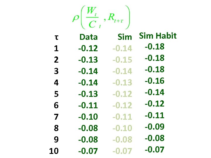τ 1 2 3 4 5 6 7 8 9 10 Data -0. 12 -0. 13 -0. 14 -0. 13 -0. 11 -0. 10 -0. 08 -0. 07 Sim Habit -0. 14 -0. 18 -0. 15 -0. 18 -0. 14 -0. 18 -0. 13 -0. 16 -0. 12 -0. 14 -0. 12 -0. 11 -0. 10 -0. 09 -0. 08 -0. 07

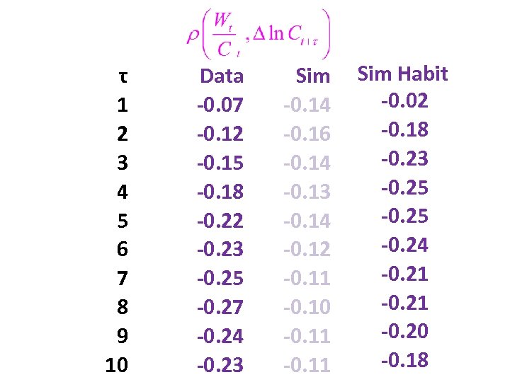τ 1 2 3 4 5 6 7 8 9 10 Data -0. 07 -0. 12 -0. 15 -0. 18 -0. 22 -0. 23 -0. 25 -0. 27 -0. 24 -0. 23 Sim -0. 14 -0. 16 -0. 14 -0. 13 -0. 14 -0. 12 -0. 11 -0. 10 -0. 11 Sim Habit -0. 02 -0. 18 -0. 23 -0. 25 -0. 24 -0. 21 -0. 20 -0. 18

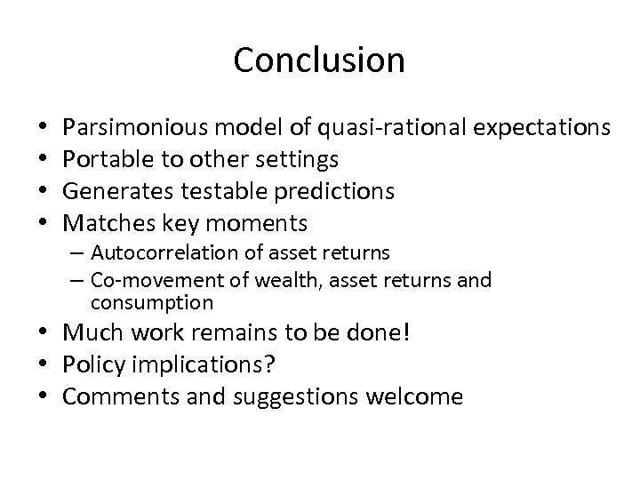Conclusion • • Parsimonious model of quasi-rational expectations Portable to other settings Generates testable predictions Matches key moments – Autocorrelation of asset returns – Co-movement of wealth, asset returns and consumption • Much work remains to be done! • Policy implications? • Comments and suggestions welcome