National Institute of Statistical Sciences Workshop on Statistics

National Institute of Statistical Sciences Workshop on Statistics and Counterterrorism G. P. Patil November 20, 2004 New York University 1

2

3

4

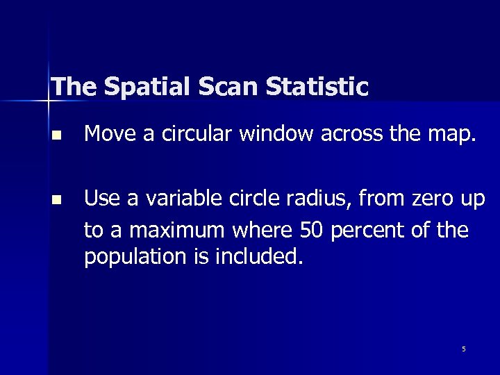The Spatial Scan Statistic n Move a circular window across the map. n Use a variable circle radius, from zero up to a maximum where 50 percent of the population is included. 5

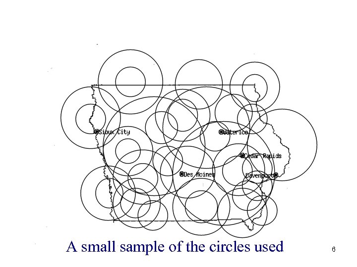A small sample of the circles used 6

Detecting Emerging Clusters n n n Instead of a circular window in two dimensions, we use a cylindrical window in three dimensions. The base of the cylinder represents space, while the height represents time. The cylinder is flexible in its circular base and starting date, but we only consider those cylinders that reach all the way to the end of the study period. Hence, we are only considering ‘alive’ clusters. 7

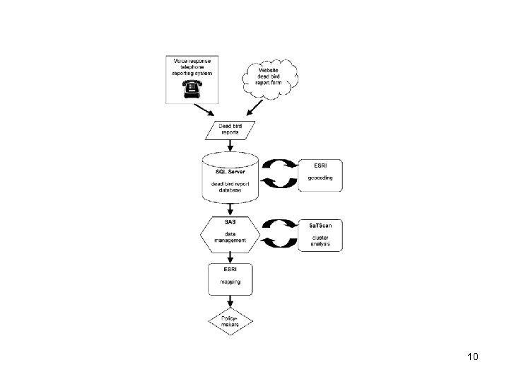
West Nile Virus Surveillance in New York City 2000 Data: Simulation/Testing of Prospective Surveillance System n 2001 Data: Real Time Implementation of Daily Prospective Surveillance n 8

West Nile Virus Surveillance in New York City Major epicenter on Staten Island Dead bird surveillance system: June 14 n Positive bird report: July 16 (coll. July 5) n Positive mosquito trap: July 24 (coll. July 7) n Human case report: July 28 (onset July 20) n 9

10

Hospital Emergency Admissions in New York City n n Hospital emergency admissions data from a majority of New York City hospitals. At midnight, hospitals report last 24 hour of data to New York City Department of Health A spatial scan statistic analysis is performed every morning If an alarm, a local investigation is conducted 11

Issues 12

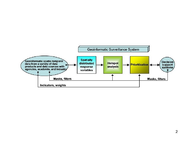
Geospatial Surveillance 13

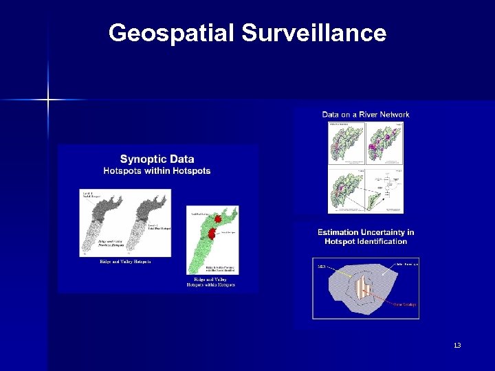
Spatial Temporal Surveillance 14

Syndromic Crisis-Index Surveillance 15

Hotspot Prioritization 16

17

National Applications n n n Biosurveillance Carbon Management Coastal Management Community Infrastructure Crop Surveillance Disaster Management Disease Surveillance Ecosystem Health Environmental Justice Sensor Networks Robotic Networks n n n n n Environmental Management Environmental Policy Homeland Security Invasive Species Poverty Policy Public Health and Environment Syndromic Surveillance Social Networks Stream Networks 18

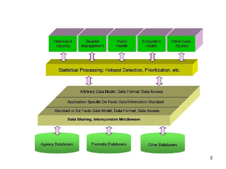
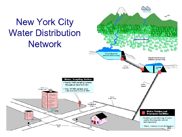
Geographic Surveillance and Hotspot Detection for Homeland Security: Cyber Security and Computer Network Diagnostics Securing the nation's computer networks from cyber attack is an important aspect of Homeland Security. Project develops diagnostic tools for detecting security attacks, infrastructure failures, and other operational aberrations of computer networks. Geographic Surveillance and Hotspot Detection for Homeland Security: Tasking of Self-Organizing Surveillance Mobile Sensor Networks Many critical applications of surveillance sensor networks involve finding hotspots. The upper level set scan statistic is used to guide the search by estimating the location of hotspots based on the data previously taken by the surveillance network. Geographic Surveillance and Hotspot Detection for Homeland Security: Drinking Water Quality and Water Utility Vulnerability New York City has installed 892 drinking water sampling stations. Currently, about 47, 000 water samples are analyzed annually. The ULS scan statistic will provide a real-time surveillance system for evaluating water quality across the distribution system. Geographic Surveillance and Hotspot Detection for Homeland Security: Surveillance Network and Early Warning Emerging hotspots for disease or biological agents are identified by modeling events at local hospitals. A time-dependent crisis index is determined for each hospital in a network. The crisis index is used for hotspot detection by scan statistic methods Geographic Surveillance and Hotspot Detection for Homeland Security: West Nile Virus: An Illustration of the Early Warning Capability of the Scan Statistic West Nile virus is a serious mosquito-borne disease. The mosquito vector bites both humans and birds. Scan statistical detection of dead bird clusters provides an early crisis warning and allows targeted public education and increased mosquito control. Geographic Surveillance and Hotspot Detection for Homeland Security: Crop Pathogens and Bioterrorism Disruption of American agriculture and our food system could be catastrophic to the nation's stability. This project has the specific aim of developing novel remote sensing methods and statistical tools for the early detection of crop bioterrorism. Geographic Surveillance and Hotspot Detection for Homeland Security: Disaster Management: Oil Spill Detection, Monitoring, and Prioritization The scan statistic hotspot delineation and poset prioritization tools will be used in combination with our oil spill detection algorithm to provide for early warning and spatial-temporal monitoring of marine oil spills and their consequences. Geographic Surveillance and Hotspot Detection for Homeland Security: Network Analysis of Biological Integrity in Freshwater Streams This study employs the network version of the upper level set scan statistic to characterize biological impairment along the rivers and streams of Pennsylvania and to identify subnetworks that are badly impaired. Center for Statistical Ecology and Environmental Statistics G. P. Patil, Director 19

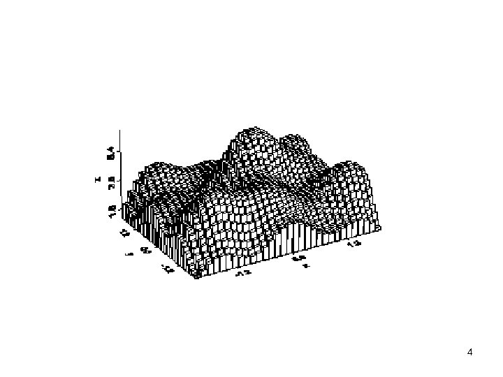
Hotspot Detection Innovation Upper Level Set Scan Statistic Attractive Features n n n n n Identifies arbitrarily shaped clusters Data-adaptive zonation of candidate hotspots Applicable to data on a network Provides both a point estimate as well as a confidence set for the hotspot Uses hotspot-membership rating to map hotspot boundary uncertainty Computationally efficient Applicable to both discrete and continuous syndromic responses Identifies arbitrarily shaped clusters in the spatial-temporal domain Provides a typology of space-time hotspots with discriminatory surveillance potential 20

Candidate Zones for Hotspots n n Goal: Identify geographic zone(s) in which a response is significantly elevated relative to the rest of a region A list of candidate zones Z is specified a priori – This list becomes part of the parameter space and the zone must be estimated from within this list – Each candidate zone should generally be spatially connected, e. g. , a union of contiguous spatial units or cells – Longer lists of candidate zones are usually preferable – Expanding circles or ellipses about specified centers are a common method of generating the list 21

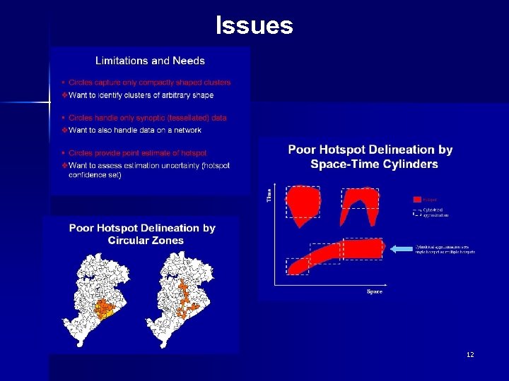
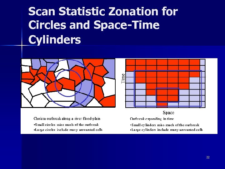Scan Statistic Zonation for Circles and Space-Time Cylinders 22

ULS Candidate Zones n n Question: Are there data-driven (rather than a priori) ways of selecting the list of candidate zones? Motivation for the question: A human being can look at a map and quickly determine a reasonable set of candidate zones and eliminate many other zones as obviously uninteresting. Can the computer do the same thing? A data-driven proposal: Candidate zones are the connected components of the upper level sets of the response surface. The candidate zones have a tree structure (echelon tree is a subtree), which may assist in automated detection of multiple, but geographically separate, elevated zones. Null distribution: If the list is data-driven (i. e. , random), its variability must be accounted for in the null distribution. A new list must be developed for each simulated data set. 23

ULS Scan Statistic n Data-adaptive approach to reduced parameter space 0 n Zones in 0 are connected components of upper level sets of the empirical intensity function Ga = Ya / Aa n n Upper level set (ULS) at level g consists of all cells a where Ga g Upper level sets may be disconnected. Connected components are the candidate zones in 0 n These connected components form a rooted tree under set inclusion. – Root node = entire region R – Leaf nodes = local maxima of empirical intensity surface – Junction nodes occur when connectivity of ULS changes with falling intensity level 24

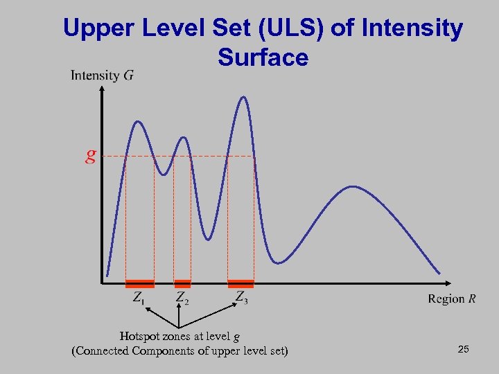Upper Level Set (ULS) of Intensity Surface Hotspot zones at level g (Connected Components of upper level set) 25

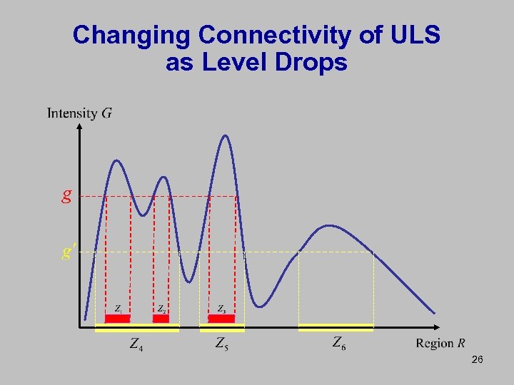Changing Connectivity of ULS as Level Drops g 26

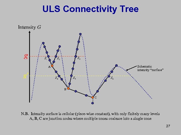ULS Connectivity Tree Schematic intensity “surface” A B C N. B. Intensity surface is cellular (piece-wise constant), with only finitely many levels A, B, C are junction nodes where multiple zones coalesce into a single zone 27

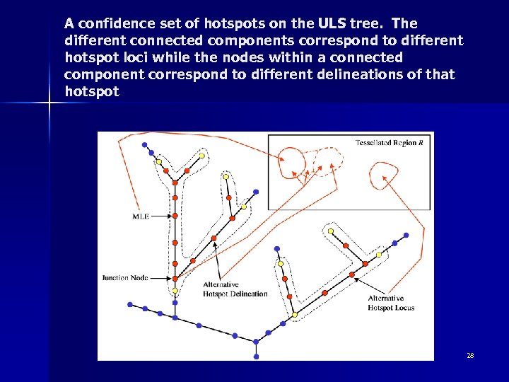A confidence set of hotspots on the ULS tree. The different connected components correspond to different hotspot loci while the nodes within a connected component correspond to different delineations of that hotspot 28

Network Analysis of Biological Integrity in Freshwater Streams 29

New York City Water Distribution Network 30

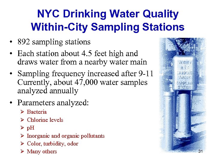NYC Drinking Water Quality Within-City Sampling Stations • 892 sampling stations • Each station about 4. 5 feet high and draws water from a nearby water main • Sampling frequency increased after 9 -11 Currently, about 47, 000 water samples analyzed annually • Parameters analyzed: Ø Ø Ø Bacteria Chlorine levels p. H Inorganic and organic pollutants Color, turbidity, odor Many others 31

Network-Based Surveillance Subway system surveillance n Drinking water distribution system surveillance n Stream and river system surveillance n Postal System Surveillance n Road transport surveillance n Syndromic Surveillance n 32

Syndromic Surveillance n Symptoms of disease such as diarrhea, respiratory problems, headache, etc n Earlier reporting than diagnosed disease n Less specific, more noise 33

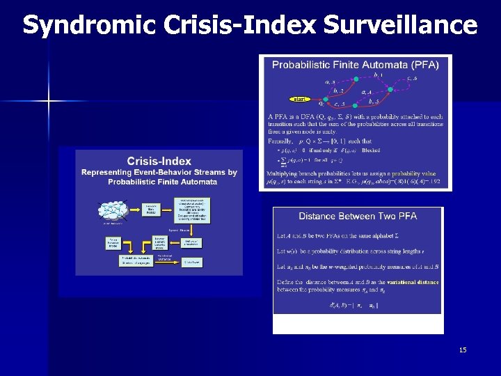
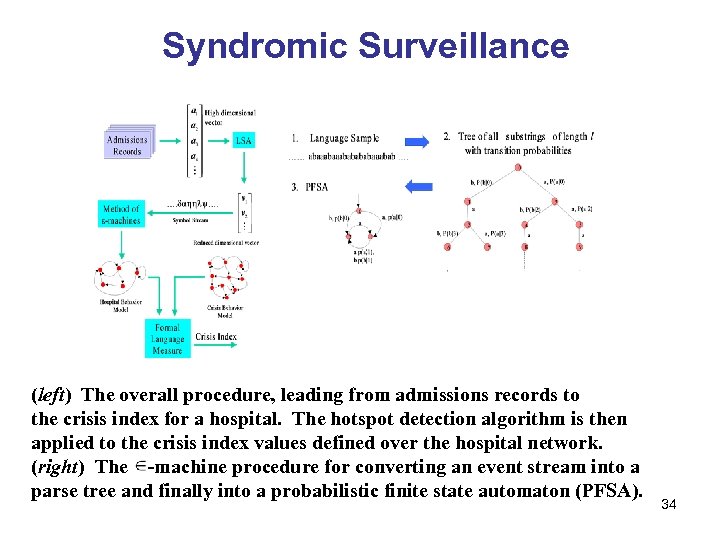Syndromic Surveillance (left) The overall procedure, leading from admissions records to the crisis index for a hospital. The hotspot detection algorithm is then applied to the crisis index values defined over the hospital network. (right) The -machine procedure for converting an event stream into a parse tree and finally into a probabilistic finite state automaton (PFSA). 34

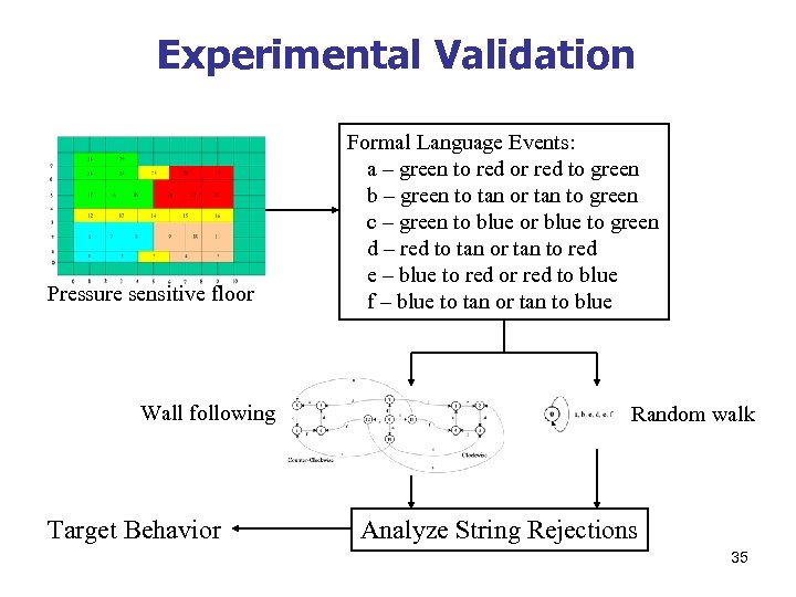Experimental Validation Pressure sensitive floor Wall following Target Behavior Formal Language Events: a – green to red or red to green b – green to tan or tan to green c – green to blue or blue to green d – red to tan or tan to red e – blue to red or red to blue f – blue to tan or tan to blue Random walk Analyze String Rejections 35

Emergent Surveillance Plexus (ESP) Surveillance Sensor Network Testbed Autonomous Ocean Sampling Network Types of Hotspots n Hotspots due to multiple, localized, stationary sources n Hotspots corresponding to areas of interest in a stationary mapped field n Time-dependent, localized hotspots n Hotspots due to moving point sources 36

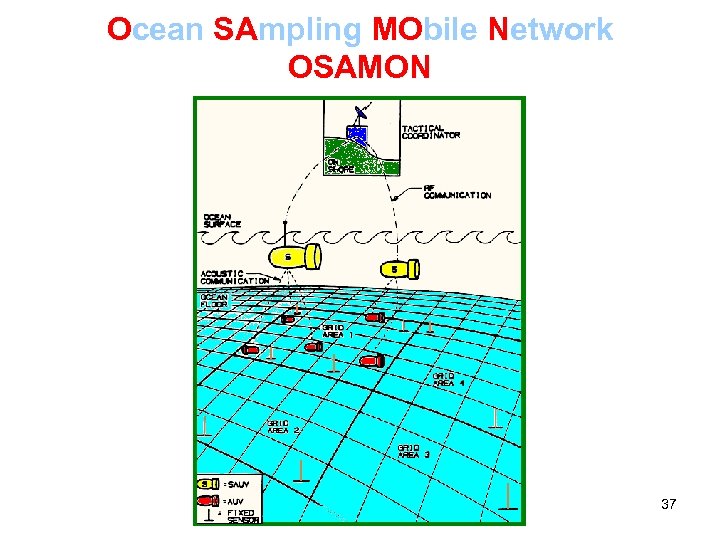Ocean SAmpling MObile Network OSAMON 37

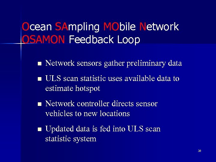Ocean SAmpling MObile Network OSAMON Feedback Loop n Network sensors gather preliminary data n ULS scan statistic uses available data to estimate hotspot n Network controller directs sensor vehicles to new locations n Updated data is fed into ULS scan statistic system 38

SAmpling MObile Networks (SAMON) Additional Application Contexts n Hotspots for radioactivity and chemical or biological agents to prevent or mitigate the effects of terrorist attacks or to detect nuclear testing n Mapping elevation, wind, bathymetry, or ocean currents to better understand protect the environment n Detecting emerging failures in a complex networked system like the electric grid, internet, cell phone systems n Mapping the gravitational field to find underground chambers or tunnels for rescue or combat missions 39

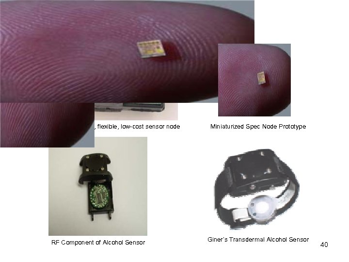Sensor Devices Mote, Smart Dust: Small, flexible, low-cost sensor node RF Component of Alcohol Sensor Miniaturized Spec Node Prototype Giner’s Transdermal Alcohol Sensor 40

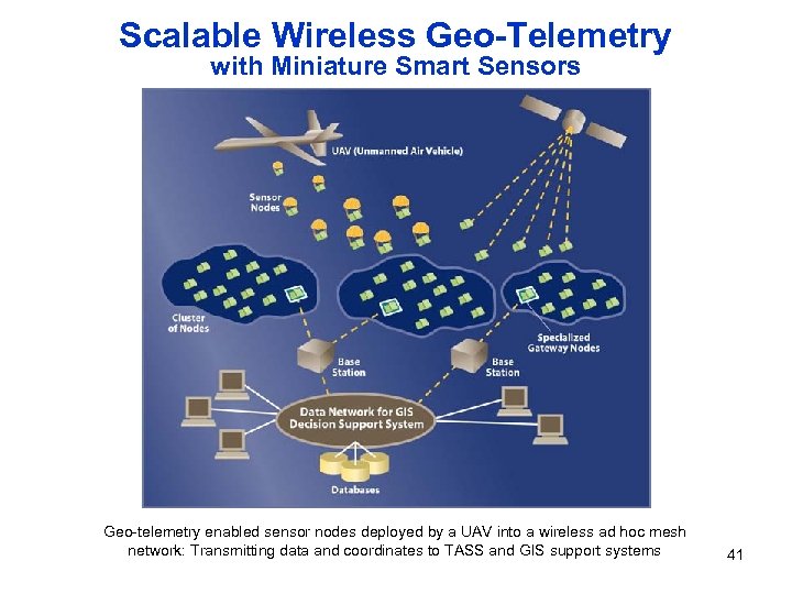Scalable Wireless Geo-Telemetry with Miniature Smart Sensors Geo-telemetry enabled sensor nodes deployed by a UAV into a wireless ad hoc mesh network: Transmitting data and coordinates to TASS and GIS support systems 41

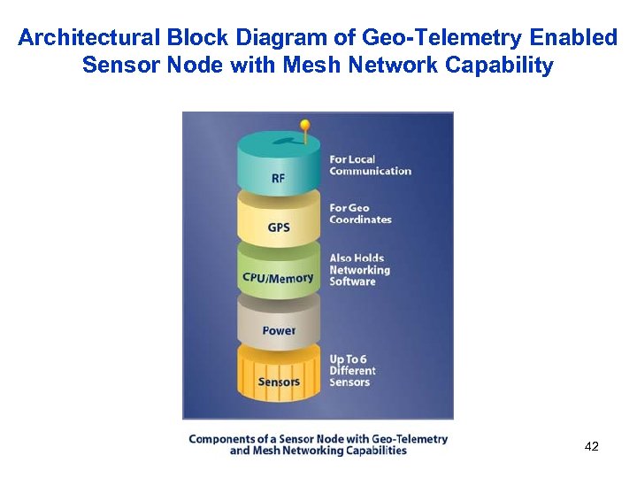Architectural Block Diagram of Geo-Telemetry Enabled Sensor Node with Mesh Network Capability 42

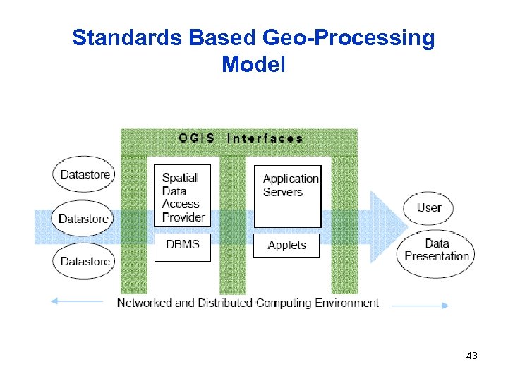Standards Based Geo-Processing Model 43

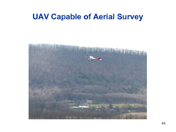UAV Capable of Aerial Survey 44

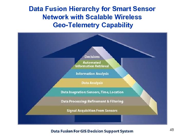Data Fusion Hierarchy for Smart Sensor Network with Scalable Wireless Geo-Telemetry Capability 45

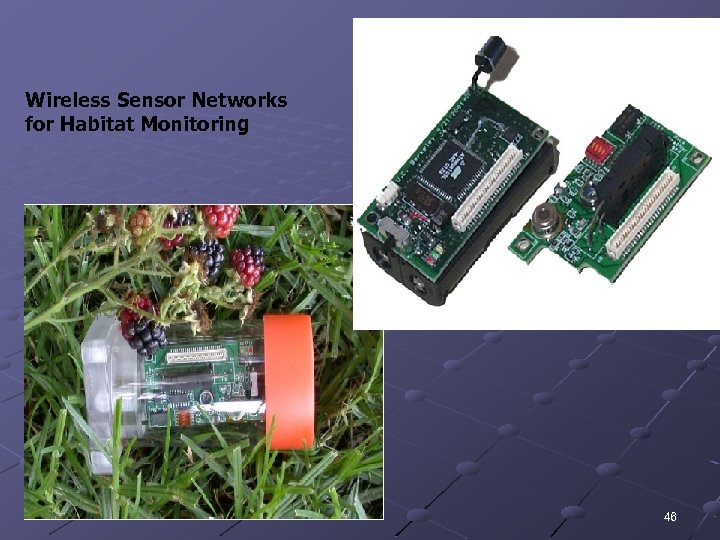Wireless Sensor Networks for Habitat Monitoring 46

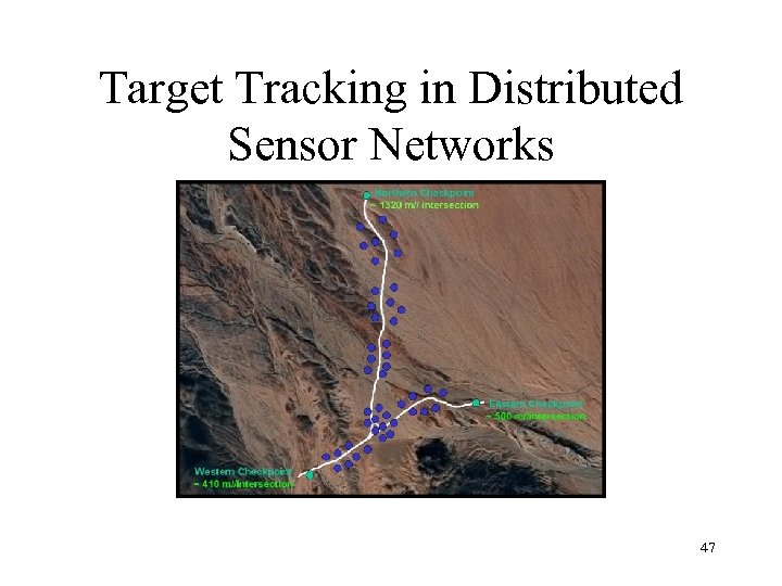Target Tracking in Distributed Sensor Networks 47

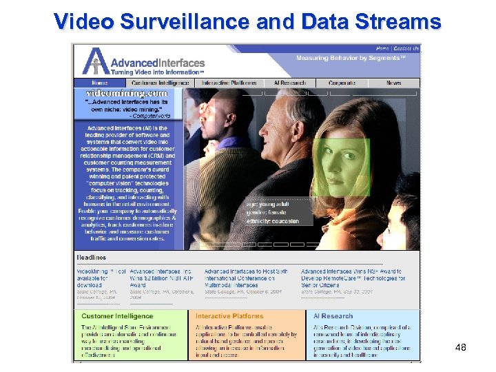Video Surveillance and Data Streams 48

Video Surveillance and Data Streams Turning Video into Information Measuring Behavior by Segments • Customer Intelligence • Enterprise Intelligence • Entrance Intelligence • Media Intelligence • Video Mining Service 49

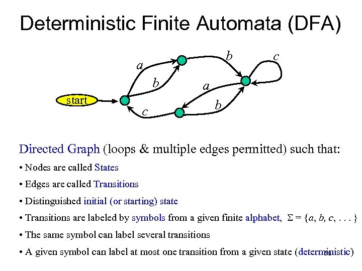Deterministic Finite Automata (DFA) b a b start c a c b Directed Graph (loops & multiple edges permitted) such that: • Nodes are called States • Edges are called Transitions • Distinguished initial (or starting) state • Transitions are labeled by symbols from a given finite alphabet, = {a, b, c, . . . } • The same symbol can label several transitions • A given symbol can label at most one transition from a given state (deterministic) 50

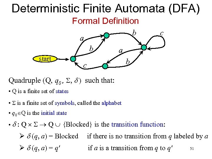Deterministic Finite Automata (DFA) Formal Definition b a b start c a b c Quadruple (Q, q 0 , , ) such that: • Q is a finite set of states • is a finite set of symbols, called the alphabet • q 0 Q is the initial state • : Q Q {Blocked} is the transition function: Ø (q, a) = Blocked if there is no transition from q labeled by a Ø (q, a) = q' if a is a transition from q to q' 51

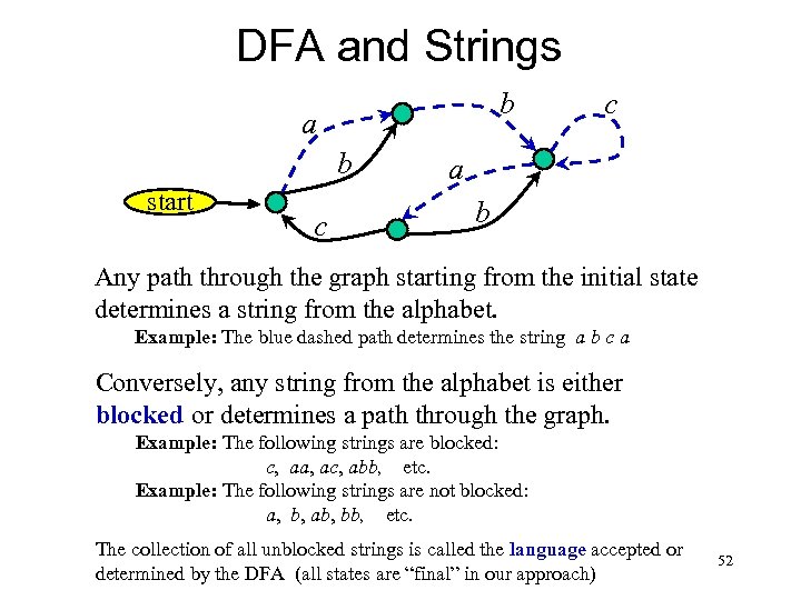DFA and Strings b a b start c c a b Any path through the graph starting from the initial state determines a string from the alphabet. Example: The blue dashed path determines the string a b c a Conversely, any string from the alphabet is either blocked or determines a path through the graph. Example: The following strings are blocked: c, aa, ac, abb, etc. Example: The following strings are not blocked: a, b, ab, bb, etc. The collection of all unblocked strings is called the language accepted or determined by the DFA (all states are “final” in our approach) 52

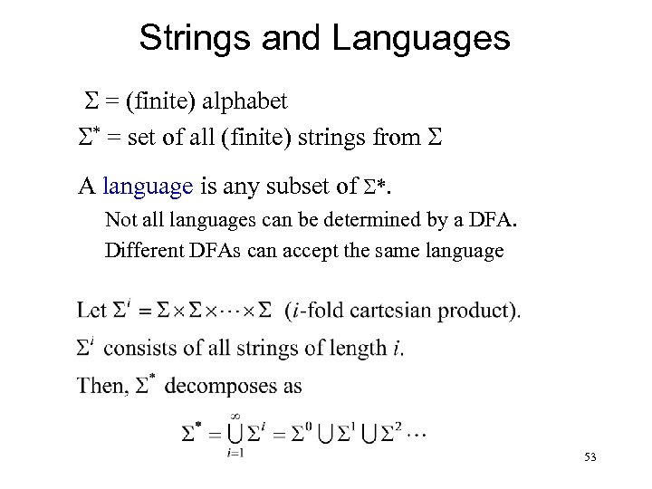Strings and Languages = (finite) alphabet * = set of all (finite) strings from A language is any subset of *. Not all languages can be determined by a DFA. Different DFAs can accept the same language 53

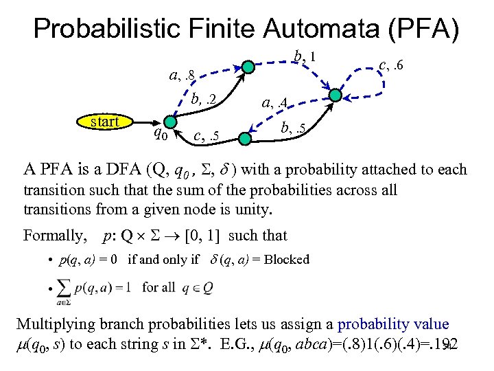Probabilistic Finite Automata (PFA) b, 1 a, . 8 b, . 2 start q 0 c, . 5 c, . 6 a, . 4 b, . 5 A PFA is a DFA (Q, q 0 , , ) with a probability attached to each transition such that the sum of the probabilities across all transitions from a given node is unity. Formally, p: Q [0, 1] such that • p(q, a) = 0 if and only if (q, a) = Blocked • Multiplying branch probabilities lets us assign a probability value (q 0, s) to each string s in *. E. G. , (q 0, abca)=(. 8)1(. 6)(. 4)=. 192 54

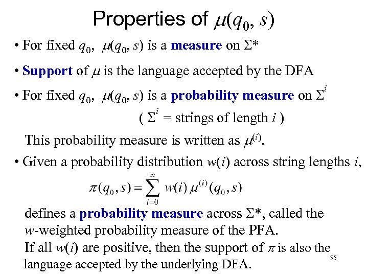Properties of (q 0, s) • For fixed q 0, (q 0, s) is a measure on * • Support of is the language accepted by the DFA • For fixed q 0, (q 0, s) is a probability measure on i i ( = strings of length i ) This probability measure is written as (i). • Given a probability distribution w(i) across string lengths i, defines a probability measure across *, called the w-weighted probability measure of the PFA. If all w(i) are positive, then the support of is also the language accepted by the underlying DFA. 55

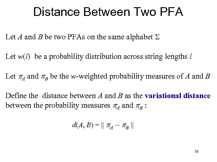Distance Between Two PFA Let A and B be two PFAs on the same alphabet Let w(i) be a probability distribution across string lengths i Let A and B be the w-weighted probability measures of A and B Define the distance between A and B as the variational distance between the probability measures A and B : d(A, B) = || A B || 56

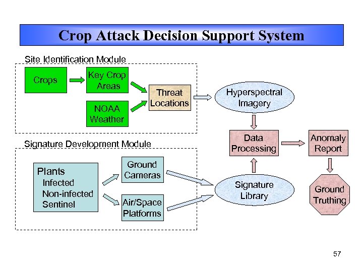Crop Attack Decision Support System Site Identification Module Crops Key Crop Areas NOAA Weather Threat Locations Signature Development Module Plants Infected Non-infected Sentinel Ground Cameras Air/Space Platforms Hyperspectral Imagery Data Processing Signature Library Anomaly Report Ground Truthing 57

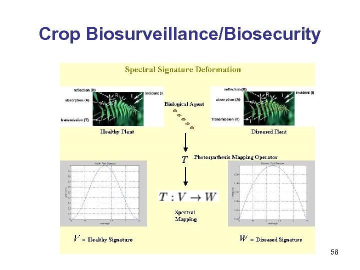Crop Biosurveillance/Biosecurity 58

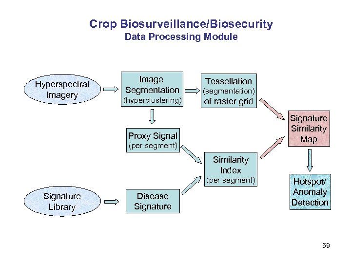Crop Biosurveillance/Biosecurity Data Processing Module Hyperspectral Imagery Image Segmentation (segmentation) (hyperclustering) of raster grid Tessellation Signature Similarity Map Proxy Signal (per segment) Similarity Index (per segment) Signature Library Disease Signature Hotspot/ Anomaly Detection 59

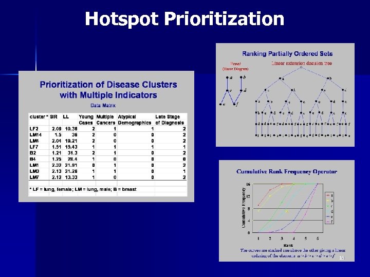
Prioritization Innovation Partial Order Set Ranking We also present a prioritization innovation. It lies in the ability for prioritization and ranking of hotspots based on multiple indicator and stakeholder criteria without having to integrate indicators into an index, using Hasse diagrams and partial order sets. This leads us to early warning systems, and also to the selection of investigational areas. 60

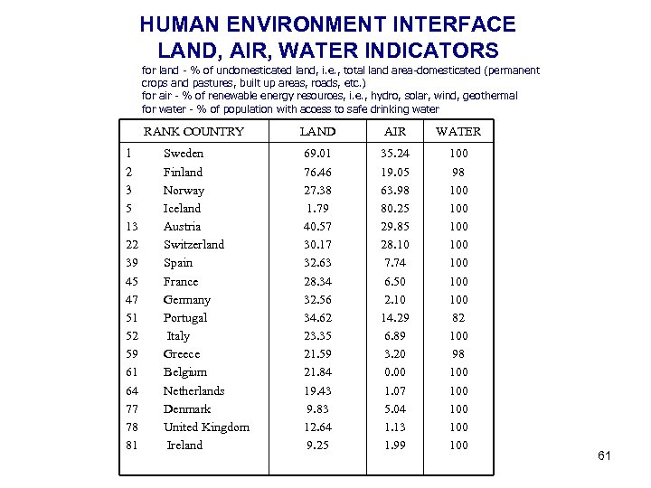HUMAN ENVIRONMENT INTERFACE LAND, AIR, WATER INDICATORS for land - % of undomesticated land, i. e. , total land area-domesticated (permanent crops and pastures, built up areas, roads, etc. ) for air - % of renewable energy resources, i. e. , hydro, solar, wind, geothermal for water - % of population with access to safe drinking water RANK COUNTRY 1 2 3 5 13 22 39 45 47 51 52 59 61 64 77 78 81 Sweden Finland Norway Iceland Austria Switzerland Spain France Germany Portugal Italy Greece Belgium Netherlands Denmark United Kingdom Ireland LAND AIR WATER 69. 01 76. 46 27. 38 1. 79 40. 57 30. 17 32. 63 28. 34 32. 56 34. 62 23. 35 21. 59 21. 84 19. 43 9. 83 12. 64 9. 25 35. 24 19. 05 63. 98 80. 25 29. 85 28. 10 7. 74 6. 50 2. 10 14. 29 6. 89 3. 20 0. 00 1. 07 5. 04 1. 13 1. 99 100 98 100 100 82 100 98 100 100 100 61

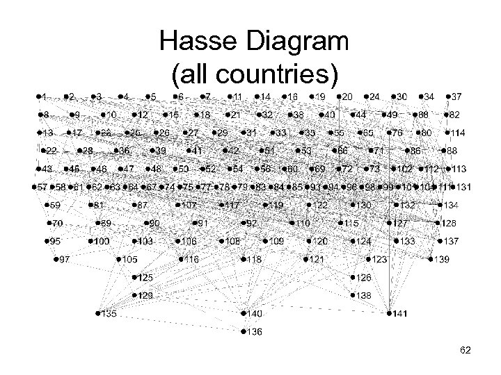Hasse Diagram (all countries) 62

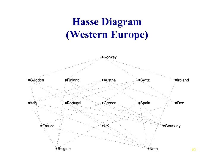Hasse Diagram (Western Europe) 63

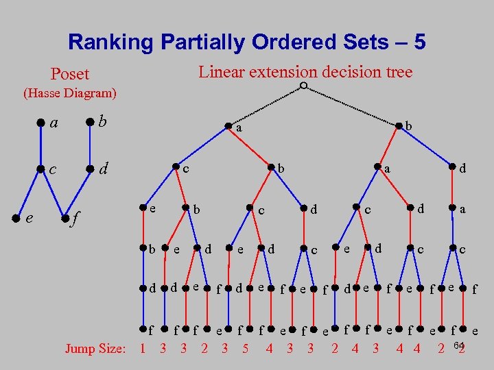Ranking Partially Ordered Sets – 5 Linear extension decision tree Poset (Hasse Diagram) a c e b d c e f b b b d e f 1 e d Jump Size: b a f f 3 3 d c d e f d d e e d e f d e d f e a c c c f d a c f e f e f e 2 3 5 4 3 3 2 4 3 4 4 2 64 2

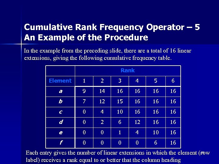Cumulative Rank Frequency Operator – 5 An Example of the Procedure In the example from the preceding slide, there a total of 16 linear extensions, giving the following cumulative frequency table. Rank Element 1 2 3 4 5 6 a 9 14 16 16 b 7 12 15 16 16 16 c 0 4 10 16 16 16 d 0 2 6 12 16 16 e 0 0 1 4 10 16 f 0 0 6 16 65 Each entry gives the number of linear extensions in which the element (row label) receives a rank equal to or better that the column heading

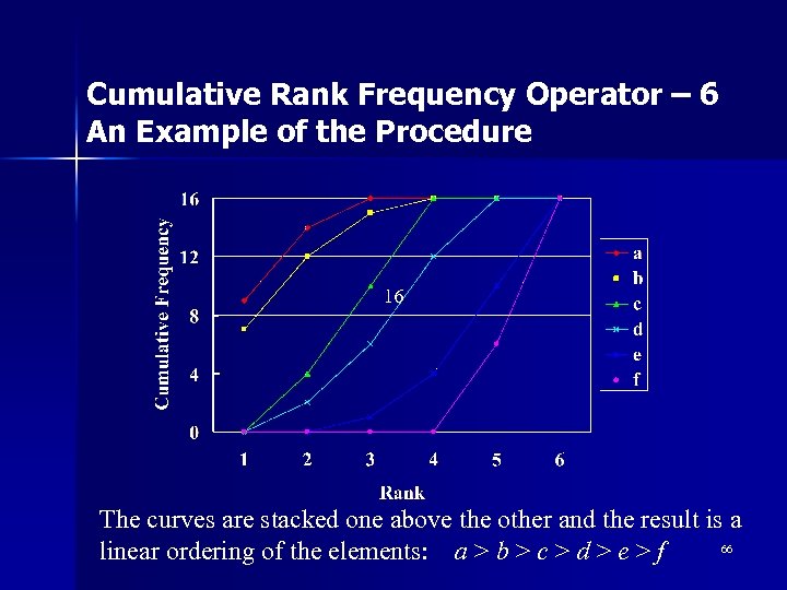Cumulative Rank Frequency Operator – 6 An Example of the Procedure 16 The curves are stacked one above the other and the result is a 66 linear ordering of the elements: a > b > c > d > e > f

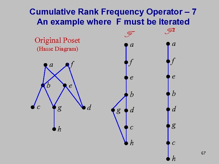Cumulative Rank Frequency Operator – 7 An example where F must be iterated F 2 F Original Poset a f b c e g h d g e b f a f e (Hasse Diagram) a b d a c g h c h 67

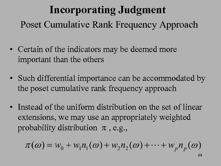Incorporating Judgment Poset Cumulative Rank Frequency Approach • Certain of the indicators may be deemed more important than the others • Such differential importance can be accommodated by the poset cumulative rank frequency approach • Instead of the uniform distribution on the set of linear extensions, we may use an appropriately weighted probability distribution , e. g. , 68

69

70

71

72

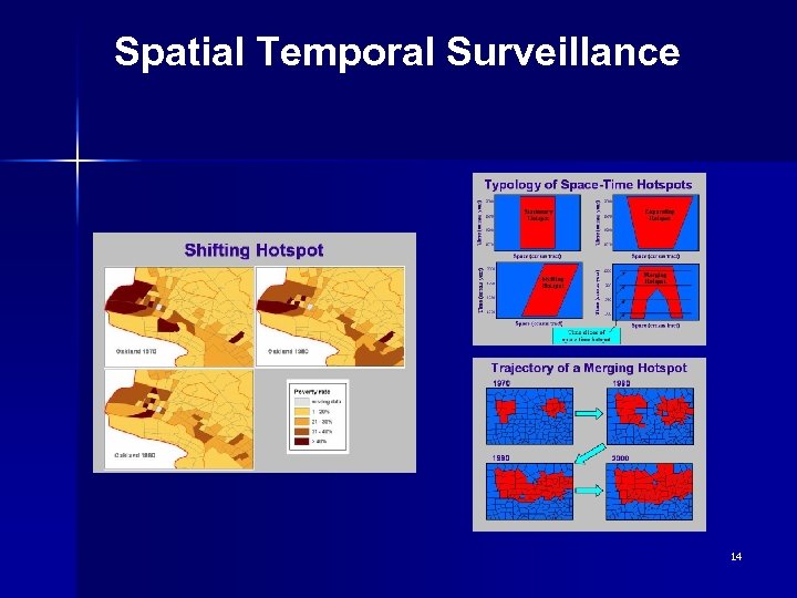
Space-Time Poverty Hotspot Typology n Federal Anti-Poverty Programs have had little success in eradicating pockets of persistent poverty n Can spatial-temporal patterns of poverty hotspots provide clues to the causes of poverty and lead to improved locationspecific anti-poverty policy ? 73

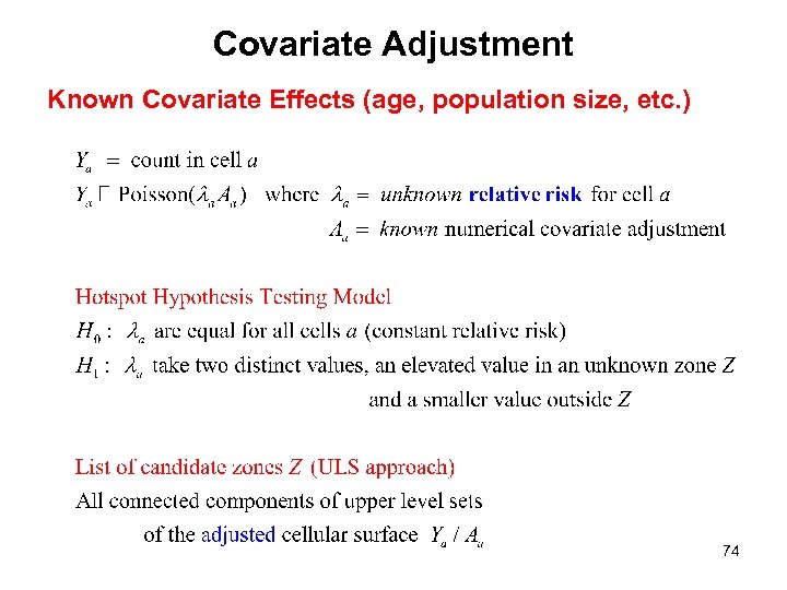Covariate Adjustment Known Covariate Effects (age, population size, etc. ) 74

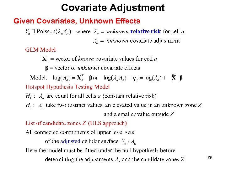Covariate Adjustment Given Covariates, Unknown Effects 75

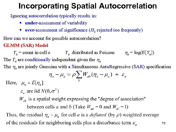Incorporating Spatial Autocorrelation Ignoring autocorrelation typically results in: § under-assessment of variability § over-assessment of significance (H 0 rejected too frequently) How can we account for possible autocorrelation? GLMM (SAR) Model Ya = count in cell a Ya distributed as Poisson a = log(E[Ya]) The Ya are conditionally independent given the a The a are jointly Gaussian with a Simultaneous Auto. Regressive (SAR) specification 76

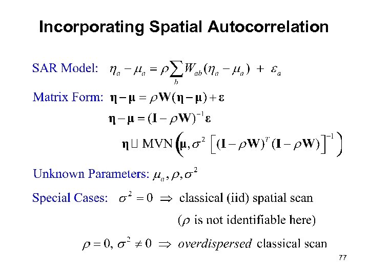Incorporating Spatial Autocorrelation 77

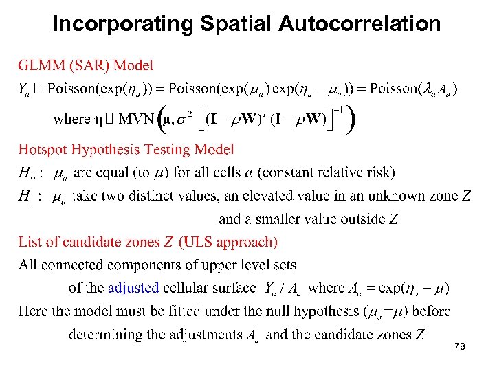Incorporating Spatial Autocorrelation 78

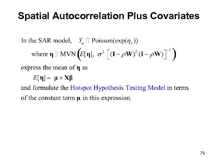Spatial Autocorrelation Plus Covariates 79

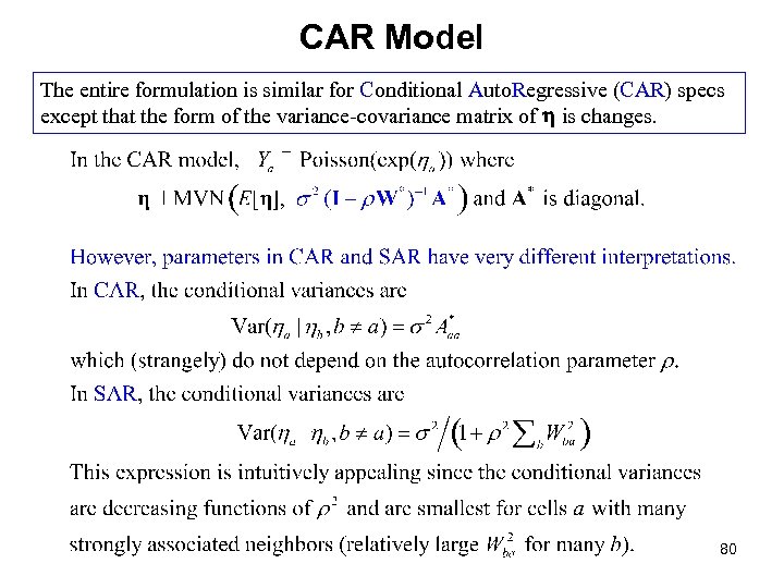CAR Model The entire formulation is similar for Conditional Auto. Regressive (CAR) specs except that the form of the variance-covariance matrix of is changes. 80

81

82