Probability Random Variables Preparatory Notes.pptx
- Количество слайдов: 35
NATCOR STOCHASTIC MODELLING (preliminary reading) Introduction to Probability & Random Variables IMPORTANT This material is designed to be viewed is two ways: 1. In ‘Slide Show’ format, to take advantage of the animations; 2. In ‘Notes Page’ format, so that you can see the accompanying notes. You might find it helps to print out the latter (to refer to) whilst NATCOR: Stochastic Modelling 2017 – Preliminary Reading viewing the former.
Overview Basic Probability • Concepts Continuous Random Variables • Definition • Laws and Notation • Probability Density Function • Conditional Probability • Probability as an Integral • Total Law of Probability • Mean and Variance Discrete Random Variables • Conditional Expectation • Definition • Probability Mass Function • Exponential Distribution • Normal Distribution • Mean and Variance • Conditional Expectation • Poisson Distribution NATCOR: Stochastic Modelling 2017 – Preliminary Reading
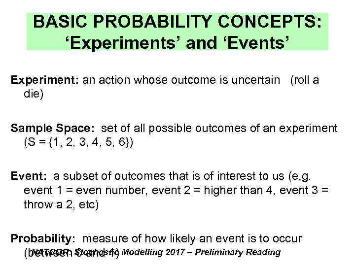
BASIC PROBABILITY CONCEPTS: ‘Experiments’ and ‘Events’ Experiment: an action whose outcome is uncertain (roll a die) Sample Space: set of all possible outcomes of an experiment (S = {1, 2, 3, 4, 5, 6}) Event: a subset of outcomes that is of interest to us (e. g. event 1 = even number, event 2 = higher than 4, event 3 = throw a 2, etc) Probability: measure of how likely an event is to occur NATCOR: 0 and 1) (between Stochastic Modelling 2017 – Preliminary Reading
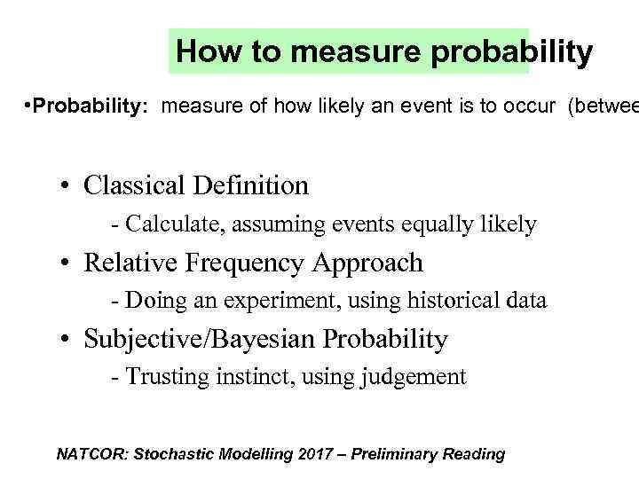
How to measure probability • Probability: measure of how likely an event is to occur (betwee • Classical Definition - Calculate, assuming events equally likely • Relative Frequency Approach - Doing an experiment, using historical data • Subjective/Bayesian Probability - Trusting instinct, using judgement NATCOR: Stochastic Modelling 2017 – Preliminary Reading
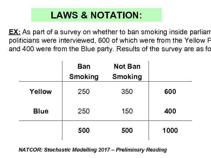
LAWS & NOTATION: EX: As part of a survey on whether to ban smoking inside parliam politicians were interviewed, 600 of which were from the Yellow P and 400 were from the Blue party. Results of the survey are as fo Ban Smoking Not Ban Smoking Yellow 250 350 600 Blue 250 150 400 500 1000 NATCOR: Stochastic Modelling 2017 – Preliminary Reading
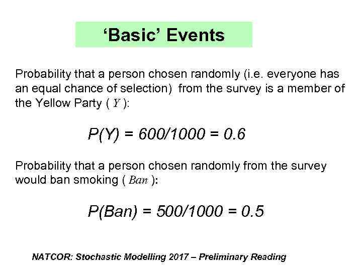
‘Basic’ Events Probability that a person chosen randomly (i. e. everyone has an equal chance of selection) from the survey is a member of the Yellow Party ( Y ): P(Y) = 600/1000 = 0. 6 Probability that a person chosen randomly from the survey would ban smoking ( Ban ): P(Ban) = 500/1000 = 0. 5 NATCOR: Stochastic Modelling 2017 – Preliminary Reading
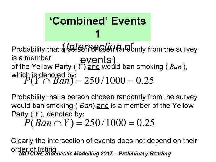
‘Combined’ Events 1 (Intersection of Probability that a person chosen randomly from the survey is a member events) of the Yellow Party ( Y ) and would ban smoking ( Ban ), which is denoted by: Probability that a person chosen randomly from the survey would ban smoking ( Ban) and is a member of the Yellow Party ( Y ), denoted by: Clearly the intersection of events does not depend on their order of listing. NATCOR: Stochastic Modelling 2017 – Preliminary Reading
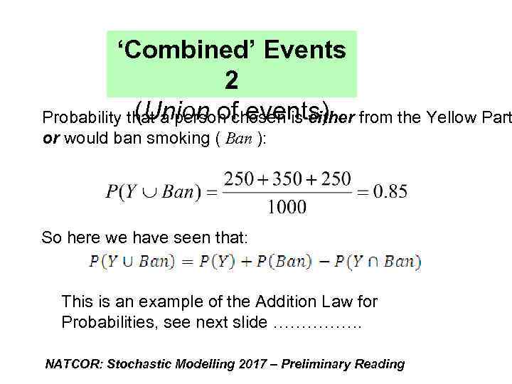
‘Combined’ Events 2 (Union of events) Probability that a person chosen is either from the Yellow Part or would ban smoking ( Ban ): So here we have seen that: This is an example of the Addition Law for Probabilities, see next slide ……………. NATCOR: Stochastic Modelling 2017 – Preliminary Reading
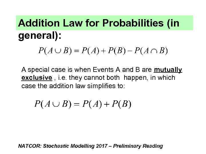
Addition Law for Probabilities (in general): A special case is when Events A and B are mutually exclusive , i. e. they cannot both happen, in which case the addition law simplifies to: NATCOR: Stochastic Modelling 2017 – Preliminary Reading
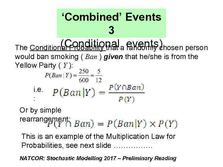
‘Combined’ Events 3 (Conditional randomly chosen person The Conditional Probability that a events) would ban smoking ( Ban ) given that he/she is from the Yellow Party ( Y ): i. e. : Or by simple rearrangement: This is an example of the Multiplication Law for Probabilities, see next slide ……………. NATCOR: Stochastic Modelling 2017 – Preliminary Reading
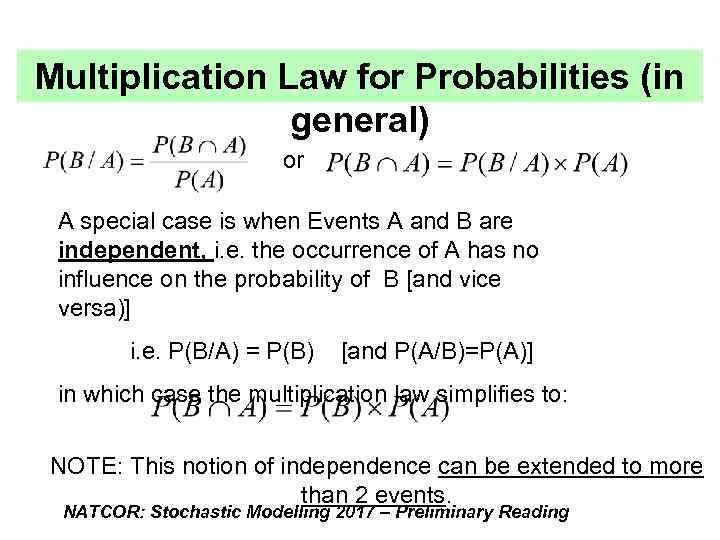
Multiplication Law for Probabilities (in general) or A special case is when Events A and B are independent, i. e. the occurrence of A has no influence on the probability of B [and vice versa)] i. e. P(B/A) = P(B) [and P(A/B)=P(A)] in which case the multiplication law simplifies to: NOTE: This notion of independence can be extended to more than 2 events. NATCOR: Stochastic Modelling 2017 – Preliminary Reading
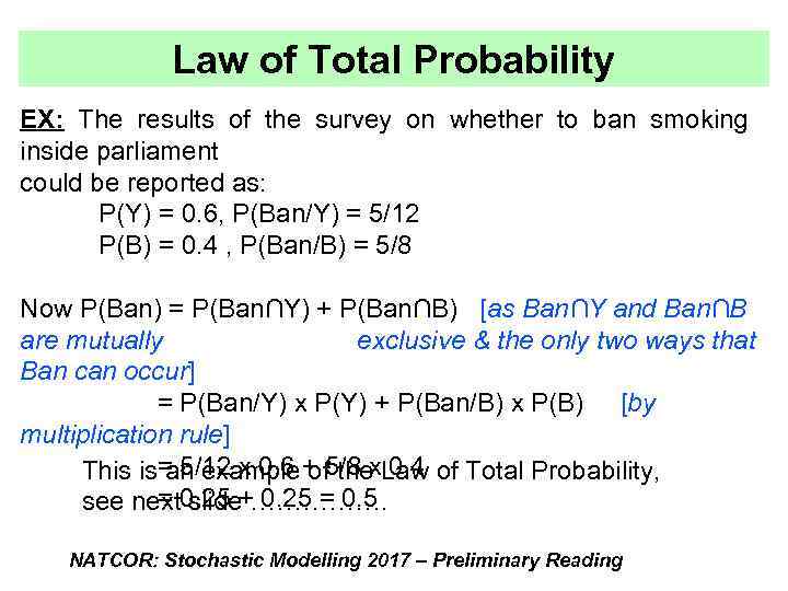
Law of Total Probability EX: The results of the survey on whether to ban smoking inside parliament could be reported as: P(Y) = 0. 6, P(Ban/Y) = 5/12 P(B) = 0. 4 , P(Ban/B) = 5/8 Now P(Ban) = P(Ban∩Y) + P(Ban∩B) [as Ban∩Y and Ban∩B are mutually exclusive & the only two ways that Ban can occur] = P(Ban/Y) x P(Y) + P(Ban/B) x P(B) [by multiplication rule] This is= 5/12 x 0. 6 + 5/8 x. Law of Total Probability, an example of the 0. 4 = slide 0. 25 = 0. 5 see next 0. 25 +……………. NATCOR: Stochastic Modelling 2017 – Preliminary Reading

Law of Total Probability in general Suppose events A 1, A 2, A 3, … An are mutually exclusive and complete (i. e. one of them must occur), then the probability of another event (B) can be calculated by weighting the conditional probabilities of B, i. e: P(B) = P(B/A 1) x P(A 1) + P(B/A 2) x P(A 2) + …P(B/An) x P(An) See another example on next slide …. . NATCOR: Stochastic Modelling 2017 – Preliminary Reading
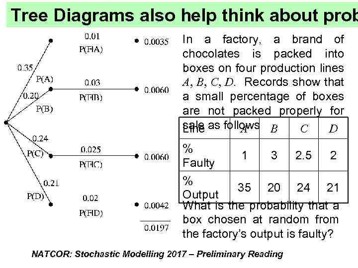
Tree Diagrams also help think about prob In a factory, a brand of chocolates is packed into boxes on four production lines A, B, C, D. Records show that a small percentage of boxes are not packed properly for sale A C D Line as follows B % 1 3 2. 5 2 Faulty % 35 20 24 21 Output What is the probability that a box chosen at random from the factory’s output is faulty? NATCOR: Stochastic Modelling 2017 – Preliminary Reading
Discrete Random Variables • A random variable is a numerical description of the outcome of an experiment. • When the values are ‘discrete’, (e. g. value shown when die is thrown, first number drawn in lottery, daily number of patients attending A&E in Lancaster), the random variable is discrete. • { For Later ***When the values are ‘continuous’ , (e. g. height of randomly selected student, temperature in Lancaster, time between patients arriving at A&E), the random variable is continuous. } NATCOR: Stochastic Modelling 2013 – Preliminary Reading • LUMS: Dept of Management Science Masters Programmes 2008/9:
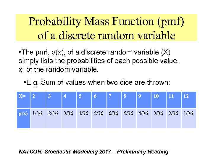
Probability Mass Function (pmf) of a discrete random variable • The pmf, p(x), of a discrete random variable (X) simply lists the probabilities of each possible value, x, of the random variable. • E. g. Sum of values when two dice are thrown: X= 2 p(x) 1/36 3 4 5 6 7 8 9 10 11 12 2/36 3/36 4/36 5/36 6/36 5/36 4/36 3/36 2/36 1/36 NATCOR: Stochastic Modelling 2017 – Preliminary Reading
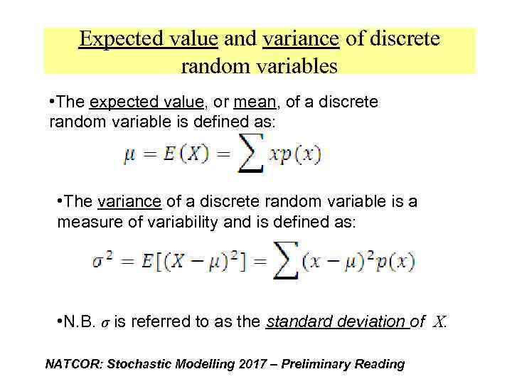
Expected value and variance of discrete random variables • The expected value, or mean, of a discrete random variable is defined as: • The variance of a discrete random variable is a measure of variability and is defined as: • N. B. σ is referred to as the standard deviation of X. NATCOR: Stochastic Modelling 2017 – Preliminary Reading

• E. g. Sum of values when two dice are thrown: X= 2 p(x) 1/36 3 4 5 6 7 8 9 10 11 12 2/36 3/36 4/36 5/36 6/36 5/36 4/36 3/36 2/36 1/36 NATCOR: Stochastic Modelling 2017 – Preliminary Reading
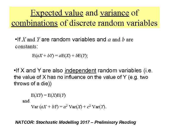
Expected value and variance of combinations of discrete random variables • If X and Y are random variables and a and b are constants: E(a. X + b. Y) = a. E(X) + b. E(Y); • If X and Y are also independent random variables (i. e. the value of X has no influence on the value of Y (e. g. two throws of a die)) E(XY) = E(X)E(Y) and Var (a. X + b. Y) = a 2 Var(X) + c 2 Var(Y). NATCOR: Stochastic Modelling 2017 – Preliminary Reading

Law of Total Probability for Expected Values of a discrete random variable Suppose events A 1, A 2, A 3, … An are mutually exclusive and complete (i. e. one of them must occur), then the expected value of a r. v. X can be calculated by weighting the conditional expected values of X, i. e. : E(X) = E(X/A 1). P(A 1) + E(X/A 2). P(A 2) + …E(X/An). P(An) • For example if 20% of the working population work at home and the remaining 80% travel an average of 10 miles to work, the overall average distance travelled to work is: E(travel to work distance) = 0 x 0. 2 + 10 x 0. 8 = 8 NATCOR: Stochastic Modelling 2017 – Preliminary Reading miles.
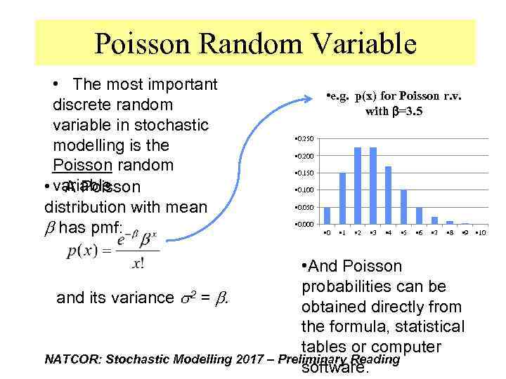
Poisson Random Variable • The most important discrete random variable in stochastic modelling is the Poisson random • variable. A Poisson distribution with mean b has pmf: • e. g. p(x) for Poisson r. v. with b=3. 5 • 0. 250 • 0. 200 • 0. 150 • 0. 100 • 0. 050 • 0. 000 • 0 • 1 • 2 • 3 • 4 • 5 • 6 • 7 • 8 • 9 • And Poisson probabilities can be 2 = b. and its variance obtained directly from the formula, statistical tables or computer NATCOR: Stochastic Modelling 2017 – Preliminary Reading software. • 10
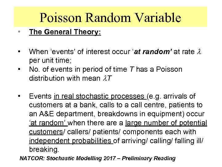
Poisson Random Variable • The General Theory: • When ‘events’ of interest occur ‘at random’ at rate l per unit time; No. of events in period of time T has a Poisson distribution with mean l. T • • Events in real stochastic processes (e. g. arrivals of customers at a bank, calls to a call centre, patients to an A&E department, breakdowns in equipment) occur ‘at random’ when there a large number of potential customers/ callers/ patients/ components each with independent probabilities of arriving/ calling/ falling ill/ breaking. NATCOR: Stochastic Modelling 2017 – Preliminary Reading
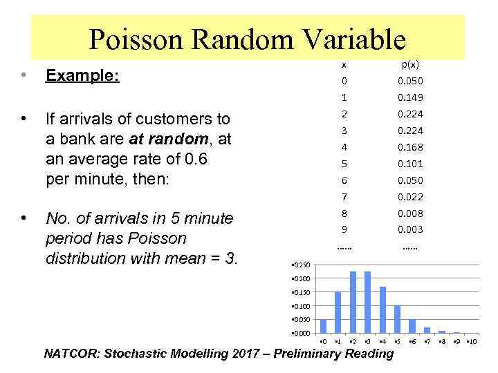
Poisson Random Variable • Example: • If arrivals of customers to a bank are at random, at an average rate of 0. 6 per minute, then: • No. of arrivals in 5 minute period has Poisson distribution with mean = 3. x 0 1 2 3 4 5 6 7 8 9 …… p(x) 0. 050 0. 149 0. 224 0. 168 0. 101 0. 050 0. 022 0. 008 0. 003 …… • 0. 250 • 0. 200 • 0. 150 • 0. 100 • 0. 050 • 0. 000 • 0 • 1 • 2 • 3 • 4 NATCOR: Stochastic Modelling 2017 – Preliminary Reading • 5 • 6 • 7 • 8 • 9 • 10
Continuous Random Variables • A random variable is a numerical description of the outcome of an experiment. • When the values are ‘continuous’ , (e. g. height of randomly selected student, temperature in Lancaster, time between patients arriving at A&E), the random variable is continuous. NATCOR: Stochastic Modelling 2017 – Preliminary Reading
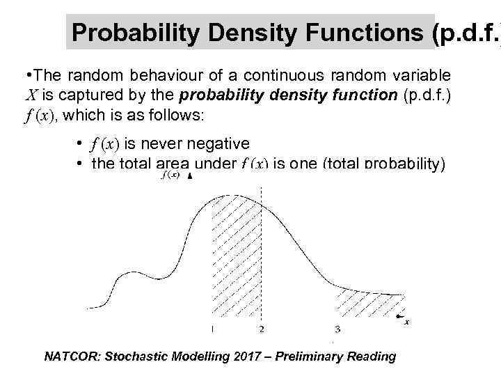
Probability Density Functions (p. d. f. ) • The random behaviour of a continuous random variable X is captured by the probability density function (p. d. f. ) f (x), which is as follows: • f (x) is never negative • the total area under f (x) is one (total probability) NATCOR: Stochastic Modelling 2017 – Preliminary Reading
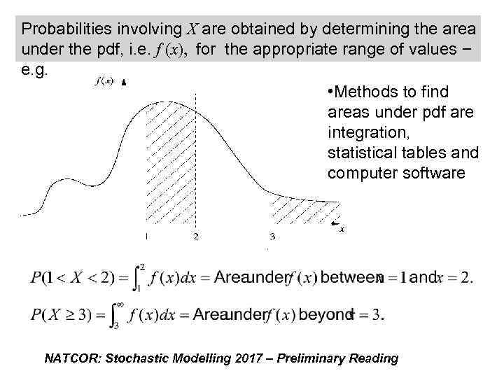
Probabilities involving X are obtained by determining the area under the pdf, i. e. f (x), for the appropriate range of values − e. g. • Methods to find areas under pdf are integration, statistical tables and computer software NATCOR: Stochastic Modelling 2017 – Preliminary Reading
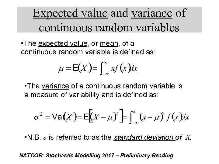
Expected value and variance of continuous random variables • The expected value, or mean, of a continuous random variable is defined as: • The variance of a continuous random variable is a measure of variability and is defined as: • N. B. σ is referred to as the standard deviation of X. NATCOR: Stochastic Modelling 2017 – Preliminary Reading
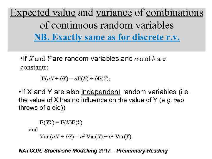
Expected value and variance of combinations of continuous random variables NB. Exactly same as for discrete r. v. • If X and Y are random variables and a and b are constants: E(a. X + b. Y) = a. E(X) + b. E(Y); • If X and Y are also independent random variables (i. e. the value of X has no influence on the value of Y (e. g. two throws of a die)) E(XY) = E(X)E(Y) and Var (a. X + b. Y) = a 2 Var(X) + c 2 Var(Y). NATCOR: Stochastic Modelling 2017 – Preliminary Reading
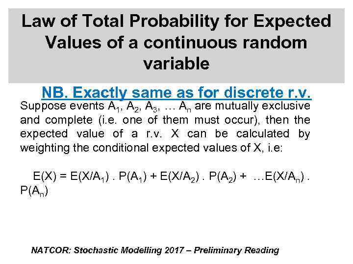
Law of Total Probability for Expected Values of a continuous random variable NB. Exactly same as for discrete r. v. Suppose events A 1, A 2, A 3, … An are mutually exclusive and complete (i. e. one of them must occur), then the expected value of a r. v. X can be calculated by weighting the conditional expected values of X, i. e: E(X) = E(X/A 1). P(A 1) + E(X/A 2). P(A 2) + …E(X/An). P(An) NATCOR: Stochastic Modelling 2017 – Preliminary Reading
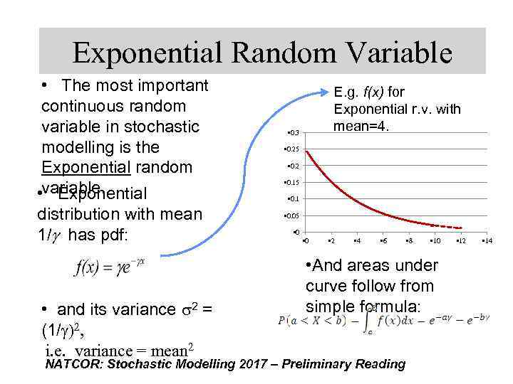
Exponential Random Variable • The most important continuous random variable in stochastic modelling is the Exponential random • variable. Exponential distribution with mean 1/g has pdf: • and its variance s 2 = (1/g)2, i. e. variance = mean 2 E. g. f(x) for Exponential r. v. with mean=4. • 0. 3 • 0. 25 • 0. 2 • 0. 15 • 0. 1 • 0. 05 • 0 • 2 • 4 • 6 • 8 • 10 • And areas under curve follow from simple formula: NATCOR: Stochastic Modelling 2017 – Preliminary Reading • 12 • 14
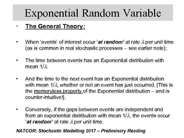
Exponential Random Variable • The General Theory: • When ‘events’ of interest occur ‘at random’ at rate l per unit time (as is common in real stochastic processes – see earlier note); • The time between events has an Exponential distribution with mean 1/l. • And the time to the next event has an Exponential distribution with mean 1/l, whether or not an event has just occurred. [This is the memoryless property of the Exponential distribution – and is counter-intuitive!]. • Conversely, if the gaps between events are independent and from an exponential distribution with mean 1/l, the events occur ‘at random’ at rate l per unit time. NATCOR: Stochastic Modelling 2017 – Preliminary Reading
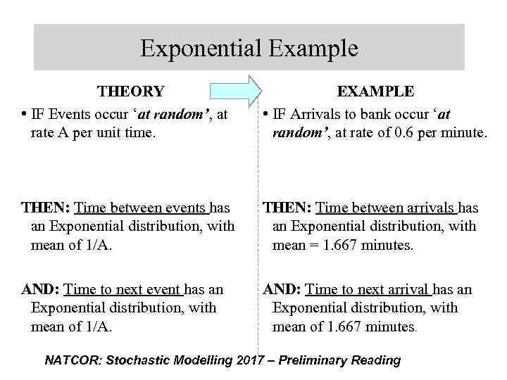
Exponential Example THEORY • IF Events occur ‘at random’, at rate A per unit time. EXAMPLE • IF Arrivals to bank occur ‘at random’, at rate of 0. 6 per minute. THEN: Time between events has an Exponential distribution, with mean of 1/A. THEN: Time between arrivals has an Exponential distribution, with mean = 1. 667 minutes. AND: Time to next event has an Exponential distribution, with mean of 1/A. AND: Time to next arrival has an Exponential distribution, with mean of 1. 667 minutes. NATCOR: Stochastic Modelling 2017 – Preliminary Reading
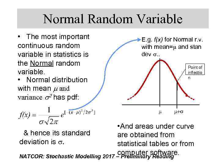
Normal Random Variable • The most important continuous random variable in statistics is the Normal random variable. • Normal distribution with mean m and variance 2 has pdf: E. g. f(x) for Normal r. v. with mean=m and stan dev s. . Point of inflectio n m m+s • And areas under curve & hence its standard are obtained from deviation is s. statistical tables or from computer software. NATCOR: Stochastic Modelling 2017 – Preliminary Reading
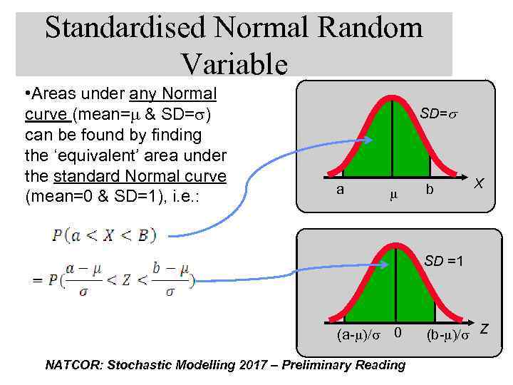
Standardised Normal Random Variable • Areas under any Normal curve (mean=m & SD=s) can be found by finding the ‘equivalent’ area under the standard Normal curve (mean=0 & SD=1), i. e. : SD= a m b X SD =1 (a-m)/s 0 NATCOR: Stochastic Modelling 2017 – Preliminary Reading (b-m)/s Z
Normal Random Variables Important (in general) because: • Many naturally occurring r. v. ’s have a Normal distribution, e. g. weights, heights … • Many useful statistics behave as Normal r. v. ’s, even if the r. v. ’s from which they derive are not Normal, e. g. Central Limit Theorem. NATCOR: Stochastic Modelling 2017 – Preliminary Reading
Probability Random Variables Preparatory Notes.pptx