Multiple Regression Models The Multiple Regression Model

Multiple Regression Models

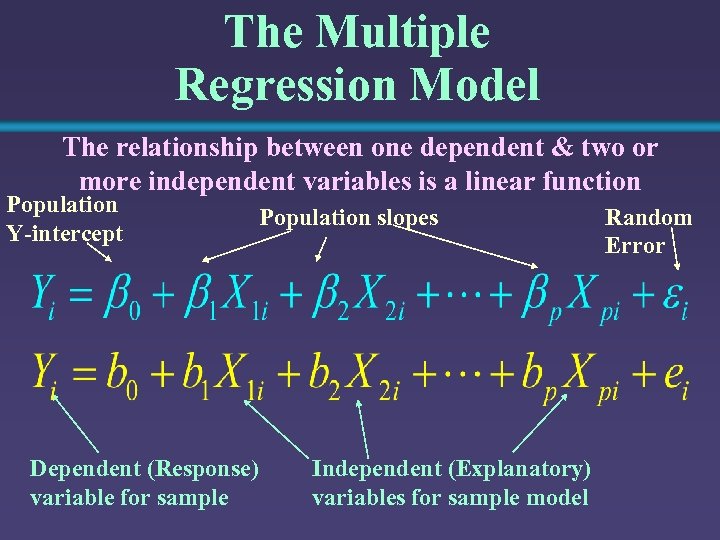The Multiple Regression Model The relationship between one dependent & two or more independent variables is a linear function Population Y-intercept Dependent (Response) variable for sample Population slopes Independent (Explanatory) variables for sample model Random Error

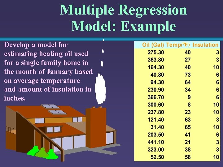Multiple Regression Model: Example Develop a model for estimating heating oil used for a single family home in the month of January based on average temperature and amount of insulation in inches. (0 F)

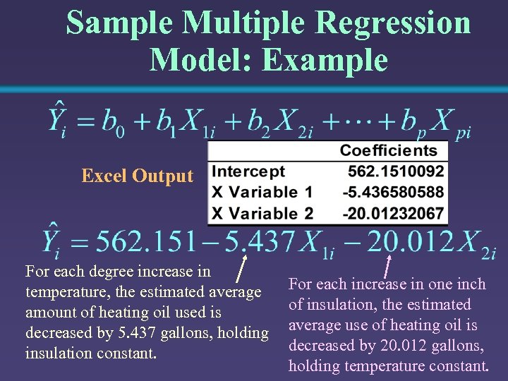Sample Multiple Regression Model: Example Excel Output For each degree increase in temperature, the estimated average amount of heating oil used is decreased by 5. 437 gallons, holding insulation constant. For each increase in one inch of insulation, the estimated average use of heating oil is decreased by 20. 012 gallons, holding temperature constant.

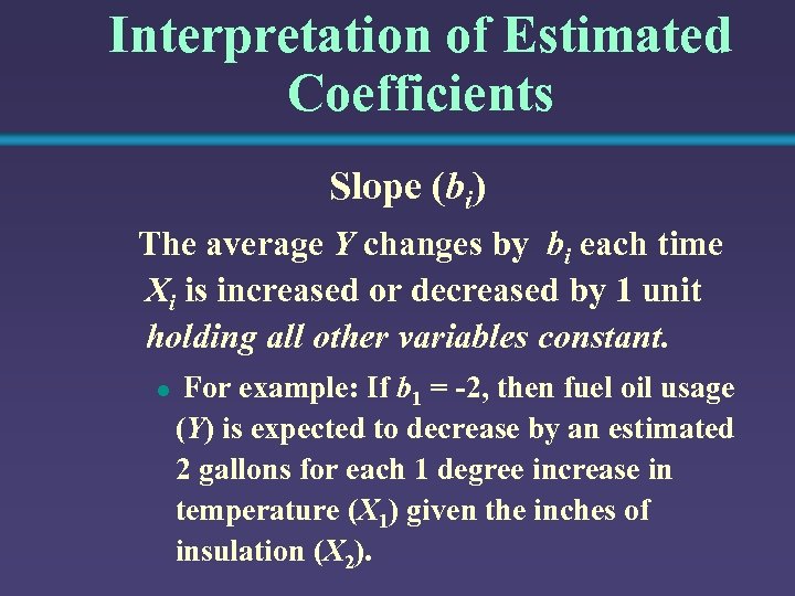Interpretation of Estimated Coefficients Slope (bi) The average Y changes by bi each time Xi is increased or decreased by 1 unit holding all other variables constant. l For example: If b 1 = -2, then fuel oil usage (Y) is expected to decrease by an estimated 2 gallons for each 1 degree increase in temperature (X 1) given the inches of insulation (X 2).

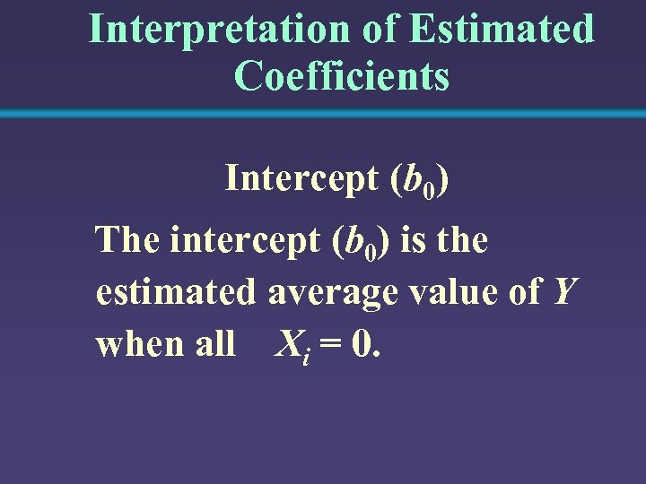Interpretation of Estimated Coefficients Intercept (b 0) The intercept (b 0) is the estimated average value of Y when all Xi = 0.

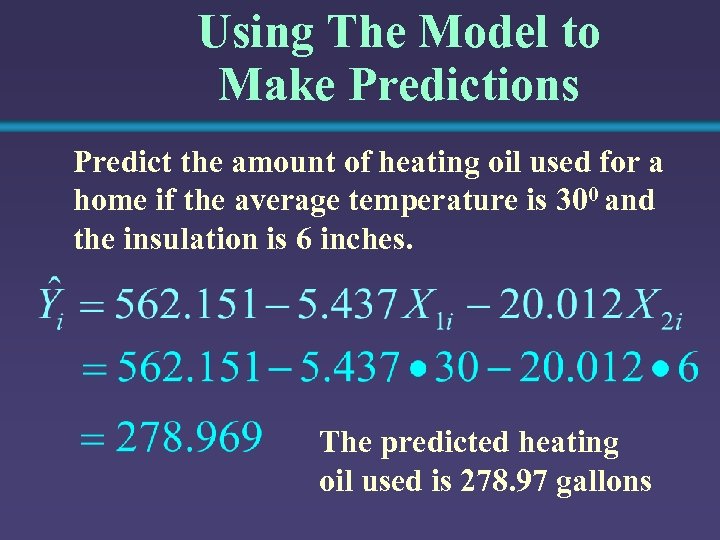Using The Model to Make Predictions Predict the amount of heating oil used for a home if the average temperature is 300 and the insulation is 6 inches. The predicted heating oil used is 278. 97 gallons

Developing the Model Checking for problems. Being sure the model passes all tests for model quality.

Identifying Problems Do all the residual tests listed for simple regression. Check for multicolinearity.

Multicolinearity • • • This occurs when there is a high correlation between the explanatory variables. This leads to unstable coefficients. The VIF used to measure colinearity (values exceeding 5 are not good and exceeding 10 are a big problem): = Coefficient of Multiple Determination of Xj with all the others

Is the fit to the data good?

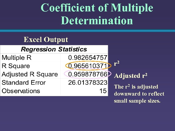Coefficient of Multiple Determination Excel Output r 2 Adjusted r 2 The r 2 is adjusted downward to reflect small sample sizes.

Do the variables collectively pass the test?

Testing for Overall Significance • Shows if there is a linear relationship between all of the X variables taken together and Y • Hypothesis: H 0: 1 = 2 = … = p = 0 (No linear relationships) H 1: At least one i 0 (At least one independent variable effects Y)

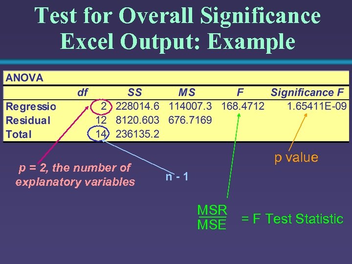Test for Overall Significance Excel Output: Example p = 2, the number of explanatory variables p value n-1 MSR MSE = F Test Statistic

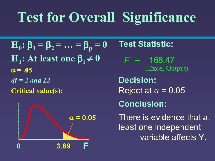Test for Overall Significance H 0: 1 = 2 = … = p = 0 H 1: At least one I 0 =. 05 df = 2 and 12 Critical value(s): Test Statistic: F 168. 47 (Excel Output) Decision: Reject at = 0. 05 Conclusion: = 0. 05 0 3. 89 F There is evidence that at least one independent variable affects Y.

Test for Significance: Individual Variables • Shows if there is a linear relationship between each variable Xi and Y. • Hypotheses: H 0: i = 0 (No linear relationship) H 1: i 0 (Linear relationship between Xi and Y)

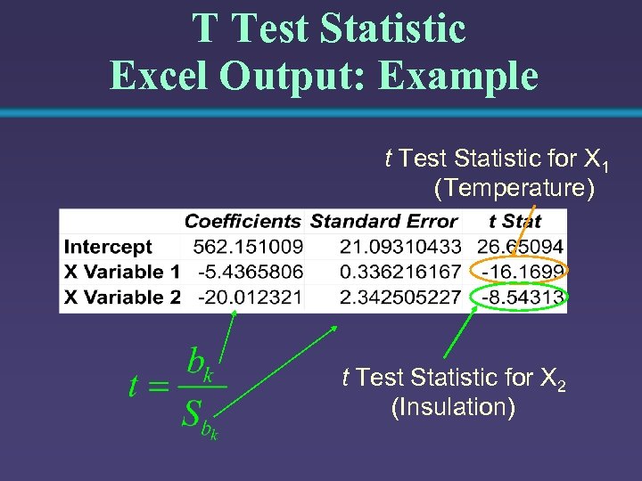T Test Statistic Excel Output: Example t Test Statistic for X 1 (Temperature) t Test Statistic for X 2 (Insulation)

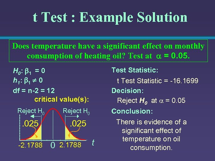t Test : Example Solution Does temperature have a significant effect on monthly consumption of heating oil? Test at = 0. 05. H 0: 1 = 0 h 1: 1 0 df = n-2 = 12 critical value(s): Reject H 0 t Test Statistic = -16. 1699 Decision: Reject H 0 at = 0. 05 Reject H 0 . 025 Test Statistic: . 025 -2. 1788 0 2. 1788 t Conclusion: There is evidence of a significant effect of temperature on oil consumption.

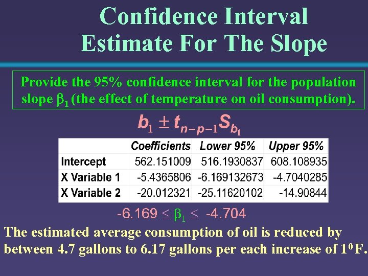Confidence Interval Estimate For The Slope Provide the 95% confidence interval for the population slope 1 (the effect of temperature on oil consumption). -6. 169 1 -4. 704 The estimated average consumption of oil is reduced by between 4. 7 gallons to 6. 17 gallons per each increase of 10 F.

Special Regression Topics

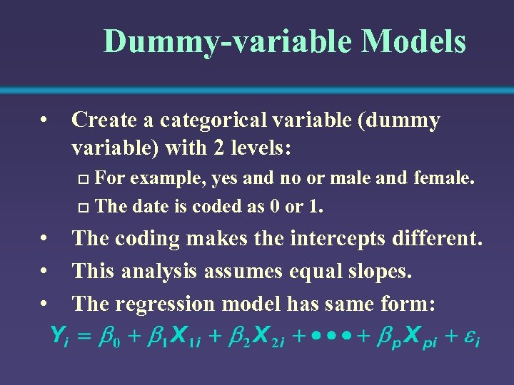Dummy-variable Models • Create a categorical variable (dummy variable) with 2 levels: For example, yes and no or male and female. o The date is coded as 0 or 1. o • • • The coding makes the intercepts different. This analysis assumes equal slopes. The regression model has same form:

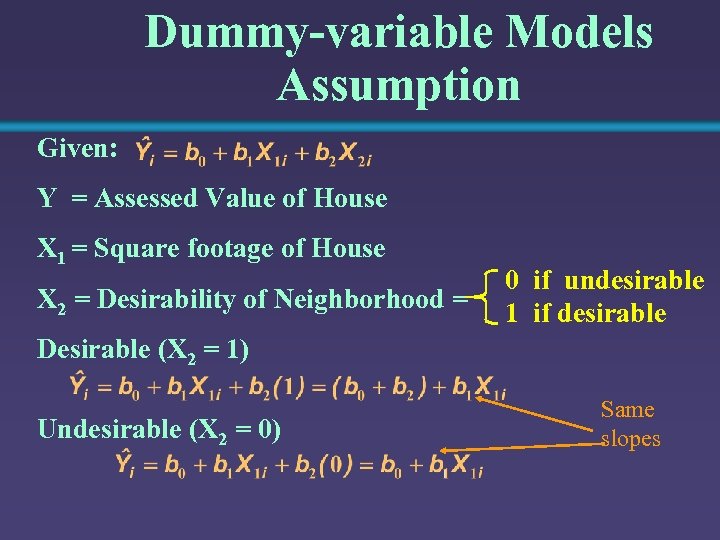Dummy-variable Models Assumption Given: Y = Assessed Value of House X 1 = Square footage of House X 2 = Desirability of Neighborhood = 0 if undesirable 1 if desirable Desirable (X 2 = 1) Undesirable (X 2 = 0) Same slopes

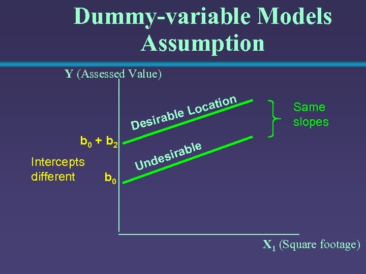Dummy-variable Models Assumption Y (Assessed Value) n e irabl Des b 0 + b 2 Intercepts different b 0 io ocat L Same slopes le irab es Und X 1 (Square footage)

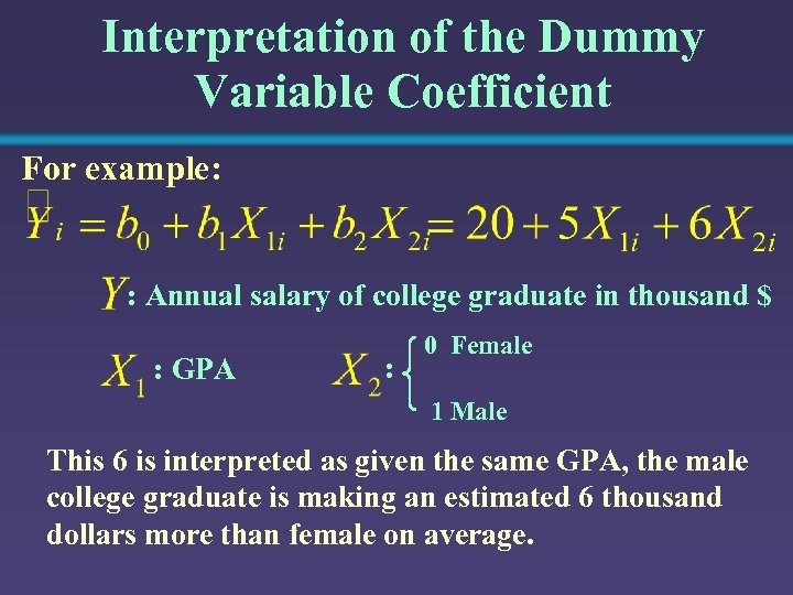Interpretation of the Dummy Variable Coefficient For example: : Annual salary of college graduate in thousand $ : GPA : 0 Female 1 Male This 6 is interpreted as given the same GPA, the male college graduate is making an estimated 6 thousand dollars more than female on average.