Multiple Regression Analysis Dr Shishen Xie Computer and

Multiple Regression Analysis Dr. Shishen Xie Computer and Math Sciences

The Simple Linear Regression Model • The simple linear regression model assumes that there is a line with y-intercept α and slope β, called the true or population regression line. When a value of the independent variable x is fixed an observation on the dependent variable y is made, y = α + βx +e • Without the random deviation e, all observed (x, y) points would fall exactly on the population regression line. The inclusion of e in the model equation recognizes that points will deviate from the line.

Simple Linear Regression Model

Multiple Regression Analysis • The general objective of regression analysis: To model the relationship between a dependent variable y and one or more independent variables. • For example, the variation of house prices can be attributed to house size, location, builder’s reputation, and other variables. • Multiple regression model includes at least two predictor variables. • Many of the concepts of simple linear regression carry over to multiple regression with little modification. • The calculations are more tedious, so a computer is an indispensable tool for multiple regression analysis.

1. Multiple Regression Models • Deterministic model: the value of y is completely determined once values of the independent variable have been specified. y = α + β 1 x 1 + β 2 x 2 + …+ βkxk • Example: In a school district, y = 38000 + 800 x 1 + 60 x 2 indicates that a teacher starts at salary ( y) of $38, 000, and receives an additional $800 per year for each year of teaching experience (x 1) and $60 per year for each unit of post college coursework (x 2). • The value of y is entirely determined by x 1 and x 2 through the deterministic formula. If two different teachers both have same number of years teaching experience (x 1) and same number of post college units (x 2) , they will have the same salary (y).

A general additive multiple regression models • A probabilistic model is more realistic in most situations: y = α + β 1 x 1 + β 2 x 2 + …+ βkxk + e • The random deviation e is assumed to be normally distributed with mean value 0 and standard deviation σ. • This implies that for fixed x 1 , x 2 , … xk values, y has a normal distribution with standard deviation σ and mean y value = α + β 1 x 1 + β 2 x 2 + …+ βkxk • The βi’s is called population regression coefficients • The deterministic portion α + β 1 x 1 + β 2 x 2 + …+ βkxk is called the population regression function.

Multiple Regression Models • Example: What factors contribute to the academic success of college sophomores? Data collected in a survey of 1000 sophomores suggests that GPA at the end of second year is related to the student’s level of interaction with faculty and staff, and to the student’s commitment to his/her major. • y = GPA at the end of the second year. x 1 = level of faculty and staff interaction (a scale from 1 to 5) x 2 = level of commitment to major (a scale from 1 to 5) • One possible population model might be α =1. 4, β 1=0. 33 and β 2= 0. 16: y = 1. 4 +. 33 x 1 + 0. 16 x 2 with σ = 0. 15. • Find mean GPA for students whose x 1=4. 2 and x 2=2. 1. • An actual y value will be within 2σ of the mean value.

Buffalo Bayou Project • We want to know how fungi population is affected by the p. H value, metal concentration, temperature, etc. of the soil at different locations along Buffalo Bayou. • In a possible multiple regression model, we can let y = fungi population x 1 = p. H value x 2 = metal concentration x 3 = temperature x 4 = location …

Polynomial Regression • Suppose that a scatterplot of the n sample (x, y) pairs has one of the appearances in the figure. A polynomial regression model is clearly more appropriate.

kth-Degree Polynomial Regression Model • y = α + β 1 x + β 2 x 2 + …+ βkxk + e is a special case of the general multiple regression model y = α + β 1 x 1 + β 2 x 2 + …+ βkxk + e with x 1= x, x 2=x 2, x 3=x 3, … xk=xk. • The most important special case other than simple linear regression (k = 1) is the quadratic regression model. y = α + β 1 x + β 2 x 2 + e • A less encountered special case is that of cubic regression: y = α + β 1 x + β 2 x 2 + β 3 x 3 + e

Interaction Between Variables • y = product from a certain chemical reaction x 1 = reaction temperature, x 2 = reaction pressure • A chemist suggests for 80 ≤ x 1 ≤ 100 and 50 ≤ x 2 ≤ 70 the probabilistic model: y = 1200 + 15 x 1 – 35 x 2 + e. • x 1 = 90: mean y value = 1200 + 15(90) – 35 x 2 = 2550 – 35 x 2 x 1 = 95: mean y value = 1200 + 15(95) – 35 x 2 = 2625 – 35 x 2 x 1 = 100: mean y value = 1200 + 15(100) – 35 x 2 = 2700 – 35 x 2 • Each graph is a straight line with the same slope – 35

Interaction Between Variables • The three lines indicates that the average change in yield when pressure x 2 is increased by 1 units is – 35, regardless of temperature. • But chemical theory suggests that the decline in average yield when pressure x 2 increases should be more rapid for a high temperature than for a low temperature.

Interaction Between Variables • Therefore, the line for a temperature x 1 = 100 should have a steeper decline than the line x 1 = 95, and that line in turn should be steeper than the one for x 1 = 90. • The previous model may not be appropriate. • A model with this property included can be y = – 4500 + 75 x 1 + 60 x 2 – x 1 x 2 + e • x 1 = 90: y = 2250 – 30 x 2 x 1 = 95: y = 2625 – 35 x 2 x 1 = 100: y = 3000 – 40 x 2

Interaction Between Variables • If the change in the mean y value associated with a 1 -unit increase in one variable depends on the value of a second variable, there is interaction between these two variables. When the variables are denoted by x 1 and x 2, such interaction can be modeled by including x 1 x 2, the product of the variables that interact, as a predictor variable. • The multiple regression model based on two independent variables x 1 and x 2 and includes an interaction predictor is y = α + β 1 x 1 + β 2 x 2 + β 3 x 1 x 2 + e. • If there are 3 independent variables, a possible model is y = α + β 1 x 1 + β 2 x 2 + β 3 x 3 + β 4 x 4 + β 5 x 5 + β 6 x 6 + e, where x 4 = x 1 x 2. x 5 = x 1 x 3 , x 6 = x 2 x 3.

Nonlinear Relationship and Transformations • Often a scatterplot exhibits a curved pattern indicating a nonlinear relationship between y and one of the variables xi. • One method to find a curve to fit the data is to find a way to transform the xi value. • A transformation involves using a simple function of a variable in place of the variable itself. For examples: ŷ = a + b ln (x) A 1 unit increase in x is associated with smaller increase or decrease in the value of y for larger x values. ŷ = a + b x½ A 1 unit increase in x is associated with smaller increase or decrease in the value of y for larger x values.

Nonlinear Multiple Regression Models • A frequently used model involving two independent variables x 1 and x 2 but k = 5 predictors is the full quadratic or complete second-order model y = α + β 1 x 1 + β 2 x 2 + β 3 x 1 x 2 + β 4 x 12 + β 5 x 22 + e When x 1 has a fixed value, the graph of the regression function for x 2 is a parabola. • Many nonlinear relationship can be put into the form y = α + β 1 x 1 + β 2 x 2 + … + βk xk + e by transforming one or more of the variables. An appropriate transformation could be suggested by theory or by various plots of data. • There also relationships that cannot be linearized by transformation, and more complicated methods of analysis must be used.

Example: Wind Chill Factor • The wind chill index combines information on air temperature and wind speed to describe how cold it really feels. The following table gives the wind chill index for various combination of air temperature and wind speed.

Example: Wind Chill Factor • y = wind chill index; x 1 = air temperature, x 2 = wind speed • Observation: The wind chill index y increases linearly with air temperature x 1 at each value of the wind speeds x 2, but the linear pattern for the different wind speeds are not parallel. • An interaction is appropriate.

Example: Wind Chill Factor • Observation: The relationship between wind chill index and wind speed is nonlinear at each of the different temperatures. • The pattern is more markedly curved at some temperatures than at others. • Therefore a transformation is necessary.

Example: Wind Chill Factor • y = wind chill index; x 1 = air temperature, x 2 = wind speed • The model used by the National Weather Service for relating wind chill index to air temperature and wind speed is mean y value = 35. 74 + 0. 621 x 1 – 35. 75 x 2′ + 0. 4275 x 1 x 2′, where x 2′ = x 20. 16 • This model incorporates a transformed x 2 to model the nonlinear relationship between wind chill index and wind speed, and an interaction term.

Example: Predictors of Writing Competence • The article “Grade Level and Gender Differences in Writing Self-Beliefs of Middle School Students” considered relating writing competence score to a number of predictor variables, including perceived value of writing and gender. • Let y = writing competence score x 1 = gender (x 1 = 0 if male, and x 1 = 1 if female) x 2 = perceived value of writing • One possible multiple regression model is y = α + β 1 x 1 + β 2 x 2 + e • Another possible model with an interaction term is y = α + β 1 x 1 + β 2 x 2 + β 3 x 1 x 2 + e

Example: Predictors of Writing Competence (no interaction) • For multiple regression model y = α + β 1 x 1 + β 2 x 2 + e when =0 (male) average y score = α + β 2 x 2 , when =1 (female) average y score = α + β 1 + β 2 x 2 , where β 1 is the coefficient is the difference in average writing score between male and female when is x 2 fixed. • The two lines are parallel with the slope both equal to β 2, although the intercept are different.

Example: Predictors of Writing Competence (interaction) • For the model with interaction, y = α + β 1 x 1 + β 2 x 2 + β 3 x 1 x 2 + e when =0 (male) average y score = α + β 2 x 2 , when =1 (female) average y score = α + β 1 + (β 2 +β 3 ) x 2 • With interaction, the lines not only have different intercepts but also have different slope (unless β 3 = 0). • The change in average writing score when x 2 increases by 1 depends on gender x 1.

2. Fitting a Model and Assessing Its Utility • Suppose a multiple regression model includes a selected set of k predictor variables x 1 , x 2 , … xk y = α + β 1 x 1 + β 2 x 2 + … + βk xk + e • It is then necessary to – estimate the model coefficients, – assess the model’s utility, and – use the estimated model to make further inferences. • A sample of n independent observations is selected, with each observation consists of k + 1 numbers: (x 1 , x 2 , … xk , y).

Definition: The Least Squares Estimates • According to the principle of least squares, the fit of a particular estimated regression function a + b 1 x 1 + b 2 x 2 + …+ bk xk to the observed data is measured by the sum of squared deviations between the observed y values and the y values predicted by the estimated function: ∑ [ y − (a + b 1 x 1 + b 2 x 2 + …+ bk xk ) ]2 The least –squares estimates of α, β 1, β 2, …, βk are those values of a, b 1, b 2, …, bk that make this sum of squared deviations as small as possible.

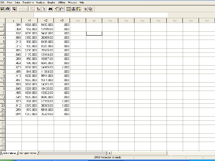
Example: Graduation Rates • One way colleges measure success is by graduation rates. We are considering the following variables: y = six-year graduation rate x 1 = median SAT score of students accepted to the college x 2 = student-related expense per full-time student (in dollars) x 3 = 1 if college has only female or only male students = 0 if college has both male and female students The data in next slide represent a random sample of 22 colleges selected from the 1037 colleges in US with enrollments less than 5000 students. Fit a linear regression model to describe the relationship between y (the six year graduation rate) and the three predictor variables.

College y x 1 x 2 x 3 Cornerstone University 0. 391 1065 9482 0 Barry University 0. 389 950 13149 0 Wilkes University 0. 532 1090 9418 0 Colgate University 0. 893 1350 26969 0 Lourdes College 0. 313 930 8489 0 Concordia University at Austin 0. 315 985 8329 0 Carleton College 0. 896 1390 29605 0 Letourneau University 0. 545 1170 13154 0 Ohio Valley College 0. 288 950 10887 0 Chadron State College 0. 469 990 6046 0 Meredith College 0. 679 1035 14889 1 Tougaloo College 0. 495 845 11694 0 Hawaii Pacific University 0. 410 1000 9911 0 University of Michigan-Dearborn 0. 497 1065 9371 0 Whitter College 0. 553 1065 14051 0 Wheaton College 0. 845 1325 18420 0 Southampton College of of Long Island 0. 465 1035 13302 0 Keene State College 0. 541 1005 8098 0 Mount St Mary’s College 0. 579 918 12999 1 Wellesley College 0. 912 1370 35393 1 Fort Lewis College 0. 298 970 5518 0 Bowdoin College 0. 891 1375 35669 0

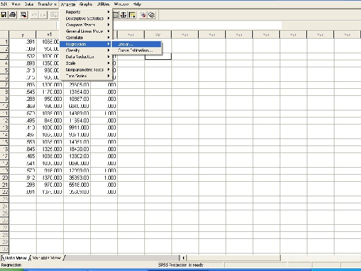
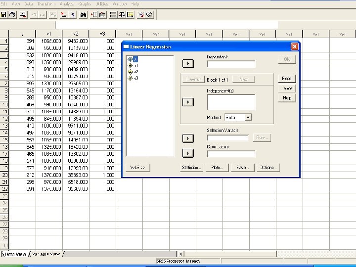
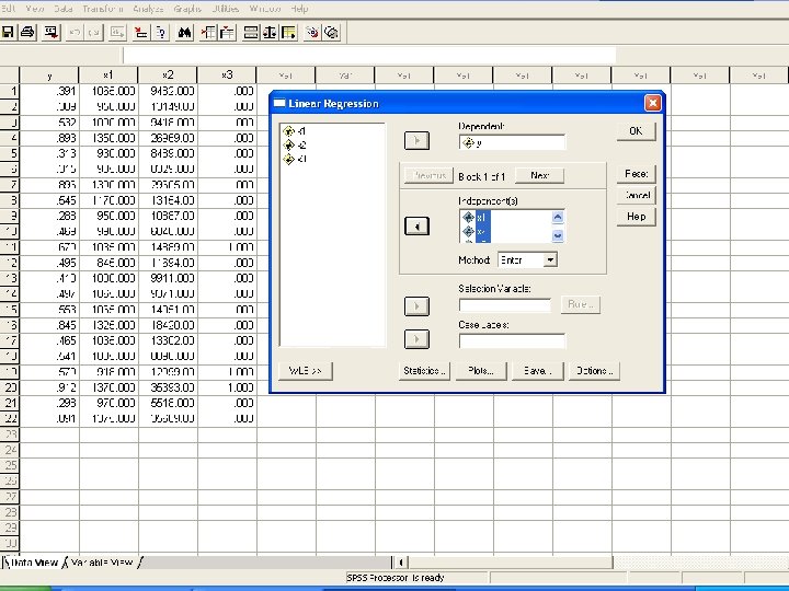
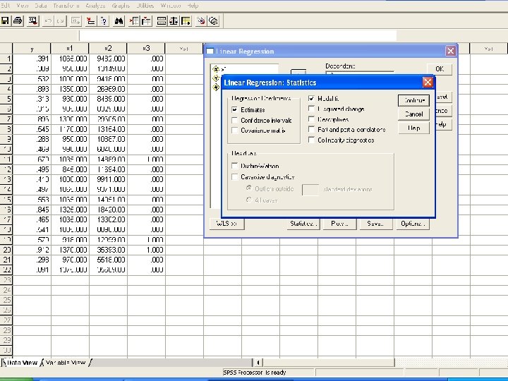
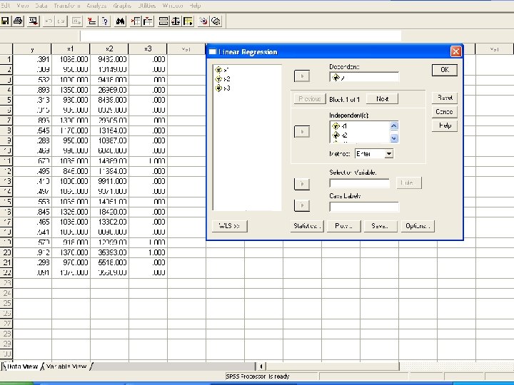
Example: Graduation Rate at Small Colleges • • In SPSS enter the data. In “Analyze”, choose the “Regression”, and then “Linear…”. Enter y as the dependent and x 1, x 2, x 3 as independent Click “Statistics” button, and a window opens. Choose “Estimates” and “Model Fit”, which should be the default. Click “Continue”. • We are back to the “Linear Regression” window. Click OK. • We can see the “Output - SPSS Viewer”. Pull the screen down we can see the “coefficients”. These are the constant term and coefficients of x variables: y = − 0. 3906 + 0. 0007602 x 1 + 0. 000006969 x 2 + 0. 125 x 3

Example: Graduation Rate at Small Colleges • The estimated mean value of y for specified x 1, x 2, and x 3 values are y = − 0. 3906 + 0. 0007602 x 1 + 0. 000006969 x 2 + 0. 125 x 3 • Use the regression function to estimate the mean six-year graduation rate of coed college with a median SAT of 1000 and an expenditure per full-time student of $11, 000. • What is the six-year graduation rate for a particular college with a median SAT of 1000 and an expenditure per full-time student of $11, 000?

Is the Model Useful? – The F Test • In the multiple regression model with regression function: y = α + β 1 x 1 + β 2 x 2 + … + βk xk, if all k coefficients β 1, β 2, …, βk are 0, there is no useful linear relationship between y and any of the predictor variables x 1, x 2, …, xk in the model. • We need to confirm the model’s utility through a formal test procedure. • When all k βi′s are 0 in the model y = α + β 1 x 1 + β 2 x 2 + … + βkxk + e and when the distribution of e is normal with mean 0 and variance σ2 for any particular values of x 1, x 2, …, xk, the model utility test for multiple regression has an F probability distribution based on df 1 = k (the number of model predictors), and df 2 = n – ( k + 1 ) (n is the sample size).

F Distribution for df 1=4, df 2 = 6: Calculated F value P-value F = 2. 16 P >. 1 F = 5. 70 . 01 < P <. 05 F = 9. 20 . 001 < P <. 01 F = 25. 03 P <. 001

Hypotheses Test • The null hypothesis, denoted by H 0, is a claim about population characteristics that is initially assumed to be true. • The alternative hypothesis, denoted by Ha, is the competing claim. • The two possible conclusions are reject H 0 , or fail to reject H 0. • α is a pre-determined significance level, which is the probability of rejecting H 0 when H 0 is true. • P-value is the area under the associated F curve to the right of the calculated F value. • H 0 should be rejected if P-value ≤ α. • H 0 should not be rejected if P-value > α.

The F Test for Utility of the Model y = α + β 1 x 1 + β 2 x 2 + … + βkxk + e • Null hypothesis: H 0: β 1= β 2 = … = βk = 0 (No useful linear relationship between y and any of the predictors. ) • Alternative hypothesis: Ha: At least one of β 1, β 2, …, βk is not 0. (A useful linear relationship between y and at least one of the predictors. ) • Test statistics: F (F is defined by a relatively complicated formula, but the calculated value of F is also available from the output of statistics software, such as SPSS. ) • Reject H 0 if P-value ≤ α. Fail to reject H 0 if P-value > α.

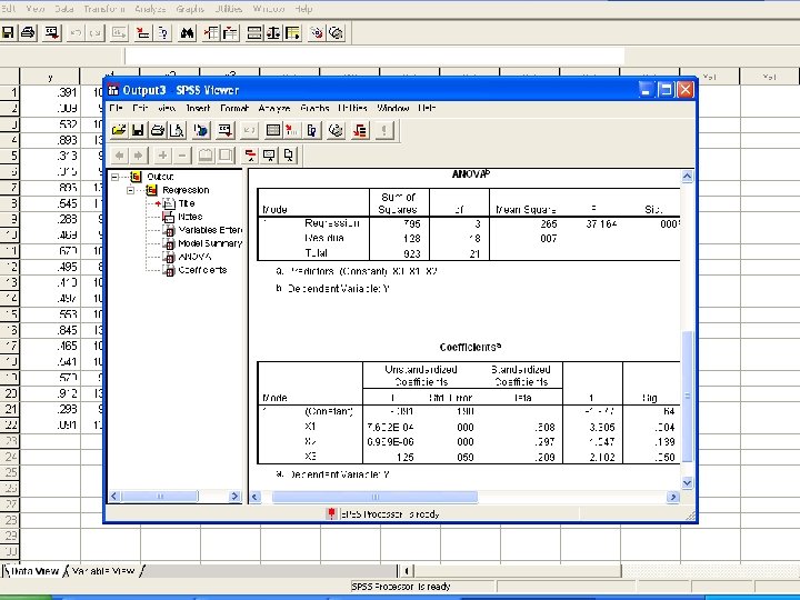
F Test for Utility of the Regression Model for the Graduation Rate of Small Colleges • The model is y = α + β 1 x 1 + β 2 x 2 + βkx 3 + e where y = six-year graduation rate, x 1 = median SAT score, x 2 = expenditure per full time student, and x 3 is an indicator if the college is coed (0) or not (1). • H 0: β 1= β 2 = β 3 = 0, Ha: At least one of β 1, β 2, β 3 is not 0. • The pre-determined significance level: α =. 05. • Test statistics: F = 37. 164 (from the “Output-SPSS Viewer” when we used SPSS to estimate the regression model. ) • df 1 = k = 3, and df 2 = n – ( k + 1 ) = 22 – (3+1) = 18. Use the F -curve Table to find P <. 001 • Reject H 0 because P < α. We thus confirm the utility of the model.

Exercise: The following data includes the price, calorie content, protein content, and fat content for a sample of 19 energy bars. What factors contribute to the price of energy bars? Use α =. 01. Price Calories Protein Fat 1. 40 180 12 3. 0 1. 28 200 14 6. 0 1. 31 210 16 7. 0 1. 10 220 13 6. 0 2. 29 220 17 11. 0 1. 15 230 14 4. 5 2. 24 240 24 10. 0 1. 99 270 24 5. 0 2. 57 320 31 9. 0 0. 94 110 5 30. 0 1. 40 180 10 4. 5 0. 53 200 7 6. 0 1. 02 220 8 5. 0 1. 13 230 9 6. 0 1. 29 230 10 2. 0 1. 28 240 10 4. 0 1. 44 260 6 5. 0 1. 27 260 7 5. 0 1. 47 290 13 6. 0

Exercises • Complete the previous example. • Do problems: 14. 2, 14. 5, 14. 7, 14. 9 14. 15, 14. 23, 14. 27, 14. 29