Multiple Regression 1 Introduction In this

Multiple Regression 1

Introduction • In this chapter, we extend the simple linear regression model. Any number of independent variables is now allowed. • We wish to build a model that fits the data better than the simple linear regression model. 2

• Computer printout is used to help us: – Assess/Validate the model • How well does it fit the data? • Is it useful? • Are any of the required conditions violated? – Apply the model • Interpreting the coefficients • Estimating the expected value of the dependent variable 3

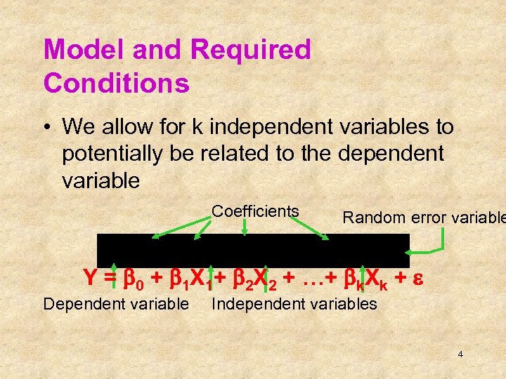Model and Required Conditions • We allow for k independent variables to potentially be related to the dependent variable Coefficients Random error variable Y = b 0 + b 1 X 1+ b 2 X 2 + …+ bk. Xk + e Dependent variable Independent variables 4

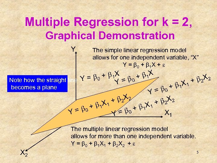Multiple Regression for k = 2, Graphical Demonstration Y The simple linear regression model allows for one independent variable, “X” Y = b 0 + b 1 X + e b 0 + b 1 X Note how the straight line Y = = + b 2 X 2 Y + b 1 X 1 becomes a plane Y = b 0 + b 2 X 2 X 1 b + b 1 X 1 b 0 + 1 Y= X 1 Y = b 0 The multiple linear regression model allows for more than one independent variable. Y = b 0 + b 1 X 1 + b 2 X 2 + e X 2 5

Required Conditions for the Error Variable • The error e is normally distributed. • The mean is equal to zero and the standard deviation is constant (se) for all possible values of the Xis. • All errors are independent. 6

Estimating the Coefficients and Assessing the Model • The procedure used to perform regression analysis: – Obtain the model coefficients and statistics using – Diagnose violations of required conditions. Try to Excel. remedy problems when identified. – Assess the model fit using statistics obtained from the sample. – If the model assessment indicates good fit to the data, use it to interpret the coefficients and generate predictions. 7

• Example 18. 1 Where to locate a new motor inn? – La Quinta Motor Inns is planning an expansion. – Management wishes to predict which sites are likely to be profitable, defined as having 50% or higher operating margin (net profit expressed as a percentage of total revenue). – Several potential predictors of profitability are: • • • Competition (room supply) Market awareness (competing motel) Demand generators (office and college) Demographics (household income) Physical quality/location (distance to downtown) 8

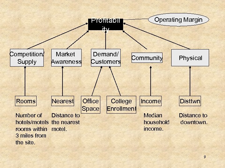Profitabil ity Competition/ Supply Rooms Market Awareness Nearest Distance to Number of hotels/motels the nearest rooms within motel. 3 miles from the site. Demand/ Customers Office Space Operating Margin Community College Income Enrollment Median household income. Physical Disttwn Distance to downtown. 9

Model and Data • Data were collected from 100 randomly-selected inns that belong to La Quinta, and ran for the following suggested model: Margin = b 0 + b 1 Rooms + b 2 Nearest + b 3 Office + Xm 18 -01 College + b 5 Income + b 6 Disttwn + e b 4 10

Excel Output This is the sample regression equation (sometimes called the prediction equation) Margin = 38. 14 - 0. 0076 Rooms +1. 65 Nearest + 0. 020 Office + 0. 21 College + 0. 41 Income - 0. 23 Disttwn 11

Model Assessment • The model is assessed using three measures: – The standard error of estimate – The coefficient of determination – The F-test of the analysis of variance • The standard error of estimates is used in the calculations for the other measures. 12

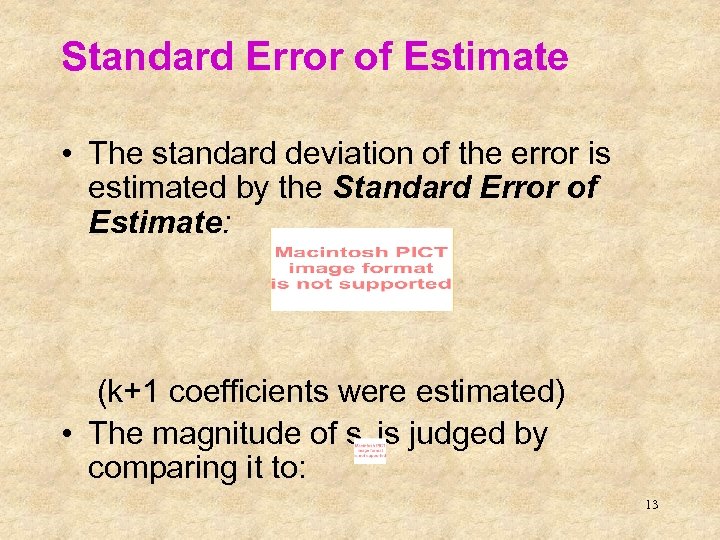Standard Error of Estimate • The standard deviation of the error is estimated by the Standard Error of Estimate: (k+1 coefficients were estimated) • The magnitude of se is judged by comparing it to: 13

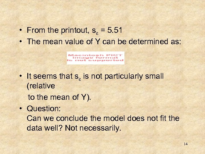• From the printout, se = 5. 51 • The mean value of Y can be determined as: • It seems that se is not particularly small (relative to the mean of Y). • Question: Can we conclude the model does not fit the data well? Not necessarily. 14

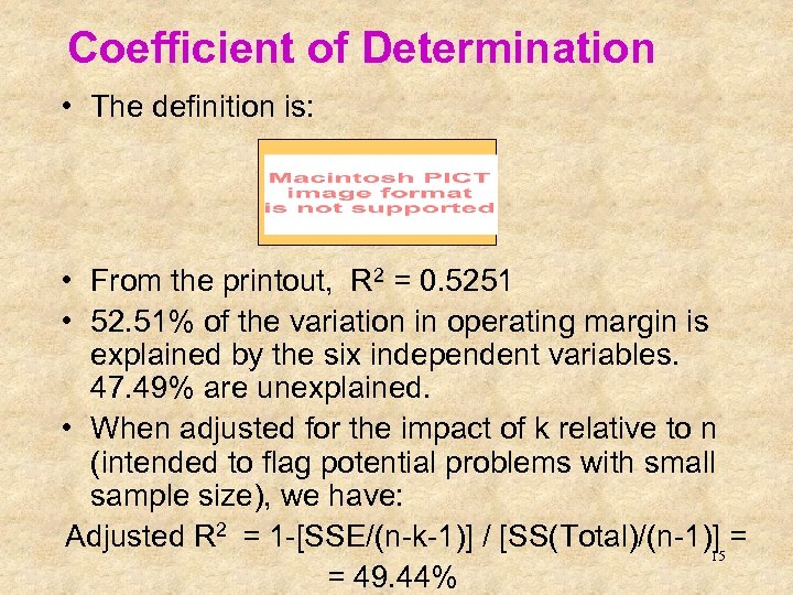Coefficient of Determination • The definition is: • From the printout, R 2 = 0. 5251 • 52. 51% of the variation in operating margin is explained by the six independent variables. 47. 49% are unexplained. • When adjusted for the impact of k relative to n (intended to flag potential problems with small sample size), we have: Adjusted R 2 = 1 -[SSE/(n-k-1)] / [SS(Total)/(n-1)] = 15 = 49. 44%

Testing the Validity of the Model • Consider the question: Is there at least one independent variable linearly related to the dependent variable? • To answer this question, we test the hypothesis: zero. H 0: b 1 = b 2 = … = b k = 0 H 1: At least one bi is not equal to • If at least one bi is not equal to zero, the model has some validity. 16 • The test is similar to an Analysis of Variance. . .

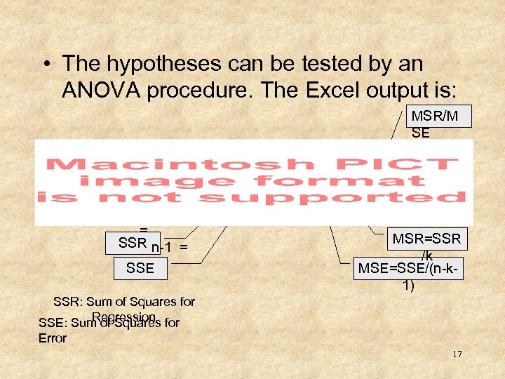• The hypotheses can be tested by an ANOVA procedure. The Excel output is: MSR/M SE k = n–k– 1 = SSR n-1 = SSE MSR=SSR /k MSE=SSE/(n-k 1) SSR: Sum of Squares for Regression SSE: Sum of Squares for Error 17

• As in analysis of variance, we have: [Total Variation in Y] = SSR + SSE. Large F indicates a large SSR; that is, much of the variation in Y is explained by the regression model. Therefore, if F is large, the model is considered valid and hence the null hypothesis should be rejected. The Rejection Region: F>Fa, k, n-k-1 18

Fa, k, n-k-1 = F 0. 05, 6, 100 -6 -1=2. 17 F = 17. 14 > 2. 17 Also, the p-value (Significance F) = 0. 0000 Reject the null hypothesis. Conclusion: There is sufficient evidence to reject the null hypothesis in favor of the alternative hypothesis: at least one of the bi is not equal to zero. Thus, at least one independent variable is linearly related to Y. 19

Interpreting the Coefficients • b 0 = 38. 14. This is the intercept, the value of Y when all the variables take the value zero. Since the data range of all the independent variables do not cover the value zero, do not interpret the intercept. • b 1 = – 0. 0076. In this model, for each additional room within 3 mile of the La Quinta inn, the operating margin decreases on average by. 0076% (assuming the other 20

• b 2 = 1. 65. In this model, for each additional mile that the nearest competitor is to a La Quinta inn, the operating margin increases on average by 1. 65%, when the other variables are held constant. • b 3 = 0. 020. For each additional 1000 sq-ft of office space, the operating margin will increase on average by. 02%, when the other variables are held constant. • b 4 = 0. 21. For each additional thousand students, the operating margin increases on average by. 21%, when the other variables are held constant. 21

• b 5 = 0. 41. For each increment of $1000 in median household income, the operating margin would increase on average by. 41%, when the other variables remain constant. • b 6 = -0. 23. For each additional mile to the downtown center, the operating margin decreases on average by. 23%, when the other variables are held constant. 22

Testing Individual Coefficients • The hypothesis for each bi is: • Excel output: H 0: b i = 0 H 1: b i ¹ 0 Ignore Test statistic d. f. = n - k -1 Insufficient Evidence 23

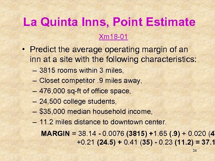La Quinta Inns, Point Estimate Xm 18 -01 • Predict the average operating margin of an inn at a site with the following characteristics: – – – 3815 rooms within 3 miles, Closet competitor. 9 miles away, 476, 000 sq-ft of office space, 24, 500 college students, $35, 000 median household income, 11. 2 miles distance to downtown center. MARGIN = 38. 14 - 0. 0076 (3815) +1. 65 (. 9) + 0. 020 (47 +0. 21 (24. 5) + 0. 41 (35) - 0. 23 (11. 2) = 37. 1 24

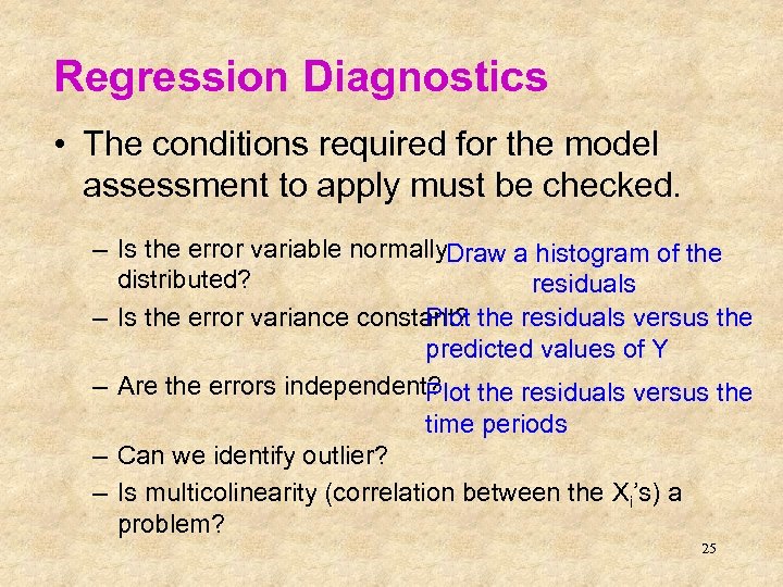Regression Diagnostics • The conditions required for the model assessment to apply must be checked. – Is the error variable normally. Draw a histogram of the distributed? residuals Plot – Is the error variance constant? the residuals versus the predicted values of Y – Are the errors independent? the residuals versus the Plot time periods – Can we identify outlier? – Is multicolinearity (correlation between the Xi’s) a problem? 25