MSC Semester 2 2003 Company Finance Richard Fairchild

MSC Semester 2, 2003: Company Finance Richard Fairchild: http: //staff. bath. ac. uk/mnsrf. Room: WH 9. 21 Email: mnsrf@bath. ac. uk 1. Topics in Investment Appraisal. 2. Risk and Return/ Portfolio Analysis. 3. Cost of Capital, Capital Structure, Firm Value. 4. Optimal Capital Structure - Agency Costs, Signalling. 5. Dividend Policy. 6. Options/Risk Management. 7. Convertible Debt. 8. Mergers and Takeovers. 1

Connections throughout the course. Investment Appraisal: Net Present Value with discount rate (cost of capital) given. Positive NPV increases value of the firm. Cost of Capital (discount rate): How do companies derive the cost of capital? – CAPM, DVM. Capital Structure and effect on Firm Value and WACC. 2

Income Statement. Finance Topics. Revenue Risk. -Variable Costs -Fixed costs Operating Leverage. -EBIT -r. D Business Risk. EBT Financial Gearing. -tax Net Income -Dividends Shareholder Risk and Return Retained earnings Dividend Policy. 3

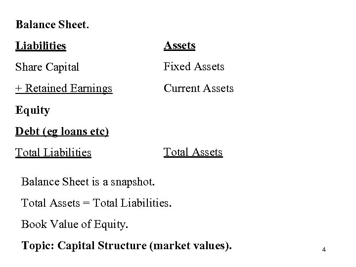Balance Sheet. Liabilities Assets Share Capital Fixed Assets + Retained Earnings Current Assets Equity Debt (eg loans etc) Total Liabilities Total Assets Balance Sheet is a snapshot. Total Assets = Total Liabilities. Book Value of Equity. Topic: Capital Structure (market values). 4

SECTION 1: Investment Appraisal. 1. Debate over Correct Method 2. - Accounting Rate of Return. - Payback. - NPV. - IRR. - POSITIVE NPV Increases Shareholder Wealth. 2. Correct Method - NPV! -Time Value of Money - Discounts all future cashflows 5

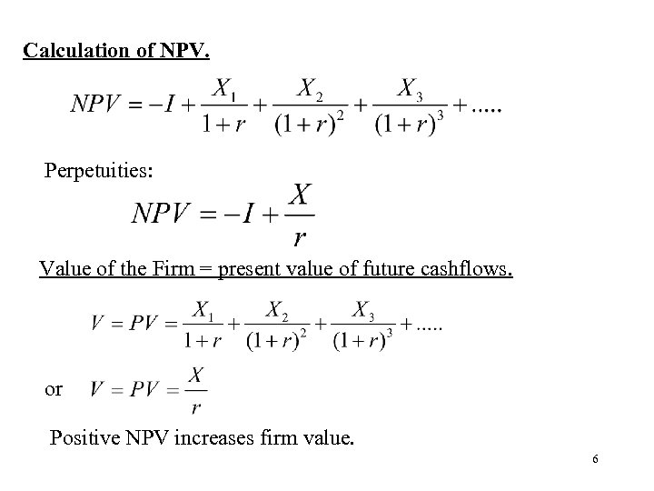Calculation of NPV. Perpetuities: Value of the Firm = present value of future cashflows. or Positive NPV increases firm value. 6

Example. Consider the following new project: -initial capital investment of £ 15 m. -it will generate sales for 5 years. - Variable Costs equal 70% of sales value. - fixed cost of project £ 200 m PA. - A feasibility study, cost £ 5000, has already been carried out. Discount Rate equals 12%. Should we take the project? 7

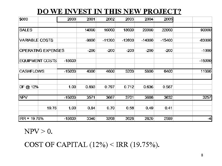DO WE INVEST IN THIS NEW PROJECT? NPV > 0. COST OF CAPITAL (12%) < IRR (19. 75%). 8

Note that if the NPV is positive, then the IRR exceeds the Cost of Capital. NPV £m 3. 3 m Discount Rate % 0 12 % 19. 7% 9

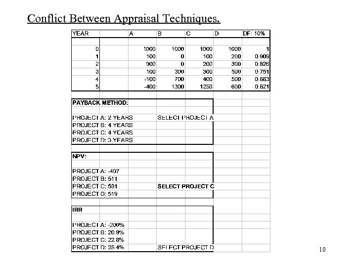Conflict Between Appraisal Techniques. 10

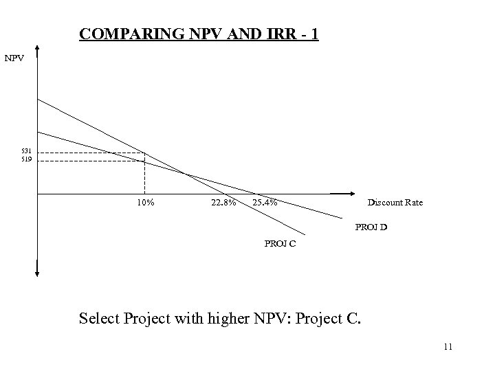COMPARING NPV AND IRR - 1 NPV 531 519 10% 22. 8% 25. 4% Discount Rate PROJ D PROJ C Select Project with higher NPV: Project C. 11

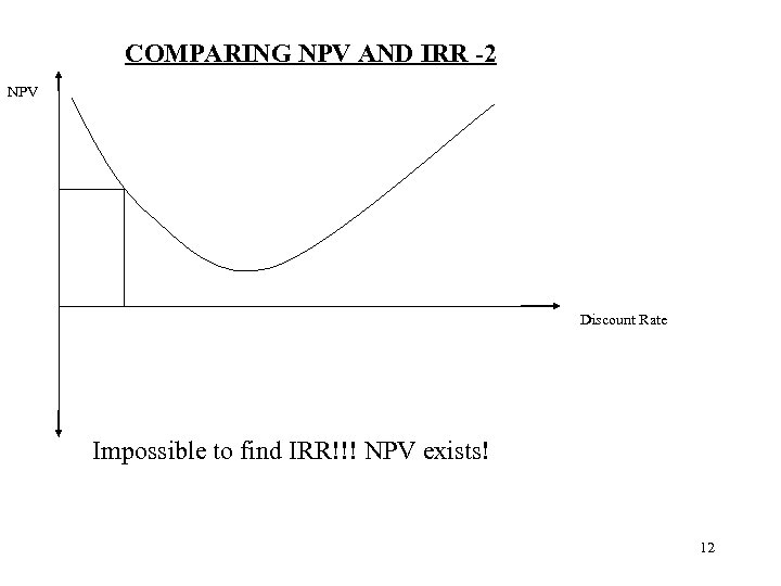COMPARING NPV AND IRR -2 NPV Discount Rate Impossible to find IRR!!! NPV exists! 12

COMPARING NPV AND IRR – 3 Discount Rate: 10% Project A : Date 0 Investment -£ 1000. Date 1 Cashflow £ 1500. NPV = £ 364. IRR = 50% Project B: - Date 0 Investment -£ 10 Date 1 Cashflow £ 18. NPV = £ 6. 36 IRR = 80%. Which Project do we take? 13

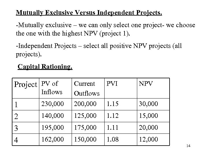Mutually Exclusive Versus Independent Projects. -Mutually exclusive – we can only select one project- we choose the one with the highest NPV (project 1). -Independent Projects – select all positive NPV projects (all projects). Capital Rationing. Project PV of NPV 230, 000 Current PVI Outflows 200, 000 1. 15 140, 000 125, 000 1. 12 15, 000 195, 000 175, 000 1. 11 20, 000 162, 000 150, 000 1. 08 12, 000 Inflows 1 2 3 4 30, 000 14

Capital Rationing And Independent Projects. The firm is limited to a capital constraint of £ 300, 000. Consider combinations of projects that maximise weighted average PVI. Eg: Projects 2 and 3: Project 1: Selecting Project 2 and 3 is superior to project 1. 15

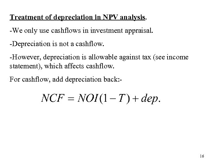Treatment of depreciation in NPV analysis. -We only use cashflows in investment appraisal. -Depreciation is not a cashflow. -However, depreciation is allowable against tax (see income statement), which affects cashflow. For cashflow, add depreciation back: - 16

Treatment of depreciation. 17

Capital Budgeting and Inflation. K is the nominal cost of capital. We require real cost of capital, where Either add inflation to the cashflow estimates, or remove inflation from the nominal cost of capital. 18

NPV and Competitive Bidding. Positive NPV => immediate increase in share price. Negative NPV => decrease in share price. Competitive bid for a supply contract, where lowest price wins (eg Space Structures exercise). Find Lowest bid price without NPV going negative. ÞFind bid price such that NPV is zero. Eg: A company is bidding for a contract to supply Y units P. A. for 3 years. Optimal bid price P? 19

The optimal bid price solves; Or: if supply forever (perpetuities) Simple to rearrange these equations to find P! 20

Decision Trees and Sensitivity Analysis. Example: From RWJ. New Project: Test and Development Phase: Investment $100 m. 0. 75 chance of success. If successful, Company can invest in full scale production, Investment $1500 m. Production will occur over next 5 years with the following cashflows. 21

Production Stage: Base Case Date 1 NPV = -1500 + = 1517 22

Decision Tree. Date 1: -1500 Date 0: -$100 P=0. 75 Success Test Failure Invest NPV = 1517 Do not Invest NPV = 0 Do not Invest P=0. 25 Do Not Test Invest NPV = -3611 Solve backwards: If the tests are successful, SEC should invest, since 1517 > 0. If tests are unsuccessful, SEC should not invest, since 0 > -3611. 23

Now move back to Stage 1. Invest $100 m now to get 75% chance of $1517 m one year later? Expected Payoff = 0. 75 *1517 +0. 25 *0 = 1138. NPV of testing at date 0 = -100 + = $890 Therefore, the firm should test the project. Sensitivity Analysis (What-if analysis or Bop analysis) Examines sensitivity of NPV to changes in underlying assumptions (on revenue, costs and cashflows). 24

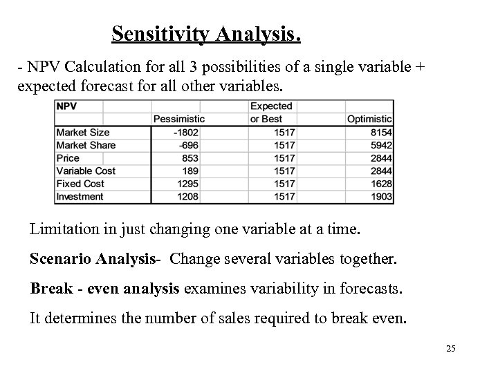Sensitivity Analysis. - NPV Calculation for all 3 possibilities of a single variable + expected forecast for all other variables. Limitation in just changing one variable at a time. Scenario Analysis- Change several variables together. Break - even analysis examines variability in forecasts. It determines the number of sales required to break even. 25

Break-even Analysis. Accounting Profit. Breakeven Point = 2091 Engines. NPV. Breakeven Point = 2315 Engines. 26

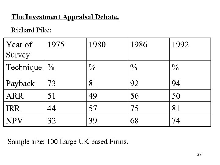The Investment Appraisal Debate. Richard Pike: Year of 1975 Survey Technique % 1980 1986 1992 % % % Payback ARR IRR NPV 81 49 57 39 92 56 75 68 94 50 81 74 73 51 44 32 Sample size: 100 Large UK based Firms. 27

Combination of Techniques: Pike 1992: Year 1975 1980 1986 1992 No Methods Single Method 2 2 0 0 0 31 (0) 24 (1) 8 (0) 4 (= PB) 34 (6) 40 (11) 29 (9) 28 (11) 3 22 (15) 24 (14) 29 (24) 32 (27) 4 11 12 34 36 Total 100 (32) 100 (38) 100 (67) 100 (74) ( ) = NPV 28

Some Reasons for usage of wrong techniques. -Managers prefer % figures => IRR, ARR -Managers don’t understand NPV/ Complicated Calculations. -Payback simple to calculate. -Short-term compensation schemes => Payback (Levy 200 – 203, Pike 1985 pg 49). Increase in Usage of correct DCF techniques: Computers. Management Education. 29

Berkovitch and Israel: Why the NPV Criterion does not Maximise NPV. -So far, NPV has been best technique, and managers use other techniques through ignorance. -In contrast, Berkovitch and Israel argue that NPV might sometimes be inefficient. -Model –Divisional Mgt identify investment opportunities. Submit capital budget requests to top mgt (HQ). -divisional mgr is an empire builder- submits bigger project with lower NPV – hides smaller project with higher NPV. -IRR or PI performs better. 30

SECTION 2: Cost Of Capital. The cost of capital = investors’ required return on their investment in a company. It provides the appropriate discount rate in NPV. Investors are risk averse. Future share prices (and returns) are risky (volatile). The higher the risk, the higher the required return. p r A B t t 31

Risk and Return. An investor’s actual return is the percentage change in price: Risk = Variability or Volatility of Returns, Var (R). We assume that Returns follow a Normal Distribution. Var(R). E(R) 32

What do we mean by Risk? The risk reflects the distribution (spread) of expected future returns. Investors are assumed to be risk-averse (don’t like risk). The higher the spread (risk), the higher the required return => current price adjusts to reflect this. Risk. Returns A B B B is riskier than A. A Time 33

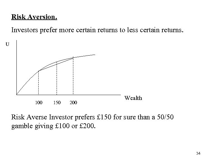Risk Aversion. Investors prefer more certain returns to less certain returns. U 100 150 200 Wealth Risk Averse Investor prefers £ 150 for sure than a 50/50 gamble giving £ 100 or £ 200. 34

Portfolio Analysis. Two Assets: Investor has proportion a of Asset X and (1 -a) of Asset Y. Combining the two assets in differing proportions. E(R) 35

Portfolio of Many assets + Risk Free Asset. E(R) Efficiency Frontier. M. * * * X * All rational investors have the same market portfolio M of risky assets, and combine it with the risk free asset. A portfolio like X is inefficient, because diversification can give higher expected return for the same risk, or the same expected return for lower risk. 36

The Effect of Diversification on Portfolio Variance. Number of Assets. An asset’s risk = Undiversifiable Risk + Diversifiable Risk = Market Risk + Specific Risk. Market portfolio consists of Undiversifiable or Market Risk only. 37

Summary of Risk and Return: Investors are assumed to be risk averse. They combine assets to diversify (reduce) risk. The more assets, the lower the specific risk. The market portfolio diversifies away all specific risk, and contains all assets in the right proportions. Implications for Investors. Current share prices (which affect expected returns) are such that the market only rewards investors for holding market risk, not specific risk. *****Implications for Individual Firms. ****** Cost of Capital (Investor’s required return) should only reflect Market Risk – (Beta – CAPM). 38

Cost of Equity. Dividend Valuation Model. This assumes that all net cashflows are paid out as dividends. Interchangeability- if we know the dividends and the market value, we can calculate the cost of equity. If we know the cost of equity and the dividends, we can calculate the market value. 39

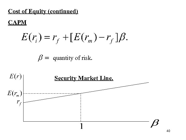Cost of Equity (continued) CAPM quantity of risk. Security Market Line. 40

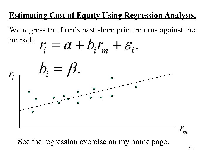Estimating Cost of Equity Using Regression Analysis. We regress the firm’s past share price returns against the market. See the regression exercise on my home page. 41

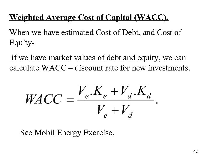Weighted Average Cost of Capital (WACC). When we have estimated Cost of Debt, and Cost of Equity if we have market values of debt and equity, we can calculate WACC – discount rate for new investments. See Mobil Energy Exercise. 42

Link to Section 3: Link between Value of the firm and NPV. Positive NPV project immediately increases current equity value (share price immediately goes up!) Pre-project announcement New capital (all equity) New project: Value of Debt Original equity holders New equity New Firm Value 43

Example: =500+500=1000. 200 60 -20 = 40. Value of Debt Original Equity New Equity Total Firm Value = 500+40 = 540 = 20 =1000+60=1060. 44

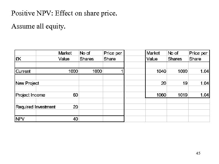Positive NPV: Effect on share price. Assume all equity. 45

SECTION 3: Value of the Firm and Capital Structure. Introduction: Value of the Firm = Value of Debt + Value of Equity = discounted value of future cashflows available to the providers of capital. (where values refer to market values). Capital Structure is the amount of debt and equity: It is the way a firm finances its investments. Unlevered firm = all-equity. Levered firm = Debt plus equity. Miller-Modigliani said that it does not matter how you split the cake between debt and equity, the value of the firm is unchanged (Irrelevance Theorem). 46

Value of the Firm = discounted value of future cashflows available to the providers of capital. -Assume Incomes are perpetuities. Miller- Modigliani Theorem: Irrelevance Theorem: Without Tax, Firm Value is independent of the Capital Structure. Note that 47

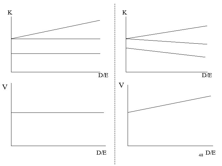K K D/E V V D/E 48 D/E

Which Cashflows do we use? Annual Income statement: Revenues 1000 Less Variable Costs 200 Less Fixed Costs 200 EBIT (=NCF) 600 Less Debt Interest (2000 @ 5%) 100 for debtholders EBT 500 Less Tax (20%) 100 Net Income (NI) 400 for equityholders 49

Calculating Levered Firm Value in our Numerical Example (see Income Statement). Let Cost of levered Equity: Market Value of Debt = 2000. Cost of risk free Debt = 5%. a) b) Now, => See Henderson Exercise. 50

MM main assumptions: - Symmetric information. -Managers unselfish- maximise shareholders wealth. -Risk Free Debt. MM assumed that investment and financing decisions were separate. Firm first chooses its investment projects (NPV rule), then decides on its capital structure. Pie Model of the Firm: D E E 51

MM irrelevance theorem- firm can use any mix of debt and equity – this is unsatisfactory as a policy tool. Searching for the Optimal Capital Structure. -Tax benefits of debt. -Asymmetric information- Signalling. -Agency Costs (selfish managers). -Debt Capacity and Risky Debt. Optimal Capital Structure maximises firm value. 52

Combining Tax Relief and Debt Capacity (Traditional View). K V D/E 53 D/E

Section 4: Optimal Capital Structure, Agency Costs, and Signalling. Agency costs - manager’s self interested actions. Signalling - related to managerial type. Debt and Equity can affect Firm Value because: - Debt increases managers’ share of equity. -Debt has threat of bankruptcy if manager shirks. - Debt can reduce free cashflow. But- Debt - excessive risk taking. 54

AGENCY COST MODELS. Jensen and Meckling (1976). - self-interested manager - monetary rewards V private benefits. - issues debt and equity. Issuing equity => lower share of firm’s profits for manager => he takes more perks => firm value Issuing debt => he owns more equity => he takes less perks => firm value 55

Jensen and Meckling (1976) V V* Slope = -1 A V 1 B If manager owns all of the equity, equilibrium point A. 56

Jensen and Meckling (1976) V V* Slope = -1 A V 1 B Slope = -1/2 B 1 B If manager owns all of the equity, equilibrium point A. If manager owns half of the equity, he will got to point B if he can. 57

Jensen and Meckling (1976) V V* Slope = -1 A B V 1 Slope = -1/2 V 2 C B 1 B 2 B If manager owns all of the equity, equilibrium point A. If manager owns half of the equity, he will got to point B if he can. 58 Final equilibrium, point C: value V 2, and private benefits B 1.

Jensen and Meckling - Numerical Example. Manager issues 100% Debt. Chooses Project B. Manager issues some Debt and Equity. Chooses Project A. Optimal Solution: Issue Debt? 59

Issuing debt increases the manager’s fractional ownership => Firm value rises. -But: Debt and risk-shifting. 60

OPTIMAL CAPITAL STRUCTURE. Trade-off: Increasing equity => excess perks. Increasing debt => potential risk shifting. Optimal Capital Structure => max firm value. V V* D/E 61

Other Agency Cost Reasons for Optimal Capital structure. Debt - bankruptcy threat - manager increases effort level. (eg Hart, Dewatripont and Tirole). Debt reduces free cashflow problem (eg Jensen 1986). 62

Agency Cost Models – continued. Effort Level, Debt and bankruptcy (simple example). Debtholders are hard- if not paid, firm becomes bankrupt, manager loses job- manager does not like this. Equity holders are soft. Effort Level High Low Required Funds Income 500 100 200 What is Optimal Capital Structure (Value Maximising)? 63

Firm needs to raise 200, using debt and equity. Manager only cares about keeping his job. He has a fixed income, not affected by firm value. a) If debt < 100, low effort. V = 100. Manager keeps job. b) If debt > 100: low effort, V < D => bankruptcy. Manager loses job. So, high effort level => V = 500 > D. No bankruptcy => Manager keeps job. High level of debt => high firm value. However: trade-off: may be costs of having high debt levels. 64

Free Cashflow Problem (Jensen 1986). -Managers have (negative NPV) pet projects. -Empire Building. => Firm Value reducing. Free Cashflow- Cashflow in excess of that required to fund all NPV projects. Jensen- benefit of debt in reducing free cashflow. 65

Jensen’s evidence from the oil industry. After 1973, oil industry generated large free cashflows. Management wasted money on unnecessary R and D. also started diversification programs outside the industry. Evidence- Mc. Connell and Muscerella (1986) – increases in R and D caused decreases in stock price. Retrenchment- cancellation or delay of ongoing projects. Empire building Management resists retrenchment. Takeovers or threat => increase in debt => reduction in free cashflow => increased share price. 66

Jensen predicts: young firms with lots of good (positive NPV) investment opportunities should have low debt, high free cashflow. Old stagnant firms with only negative NPV projects should have high debt levels, low free cashflow. Stultz (1990)- optimal level of debt => enough free cashflow for good projects, but not too much free cashflow for bad projects. 67

Income Rights and Control Rights. Some researchers (Hart (1982) and (2001), Dewatripont and Tirole (1985)) recognised that securities allocate income rights and control rights. Debtholders have a fixed first claim on the firm’s income, and have liquidation rights. Equityholders are residual claimants, and have voting rights. Class discussion paper: Hart (2001)- What is the optimal allocation of control and income rights between a single investor and a manager? How effective are control rights when there are different types of investors? Why do we observe different types of outside investors- what is 68 the optimal contract?

Conflict Benefits of Debt Costs of Debt Breaking MM Tax Relief Fin’l Distress/ Debt Capacity Agency Models JM (1976) Managerial Perks Increase Mgr’s Ownership Risk Shifting Jensen (1986) Empire Building Reduce Freecash Unspecified. Stultz Empire Building Reduce Freecash Underinvestment. Dewatripont and Tirole, Hart. Low Effort level Bankruptcy threat =>increased effort DT- Inefficient liquidations. 69

Signalling Models of Capital Structure Assymetric info: Akerlof’s (1970) Lemons Market. Akerlof showed that, under assymetric info, only bad things may be traded. His model- two car dealers: one good, one bad. Market does not know which is which: 50/50 probability. Good car (peach) is worth £ 2000. Bad car (lemon) is worth £ 1000. Buyers only prepared to pay average price £ 1500. But: Good seller not prepared to sell. Only bad car remains. Price falls to £ 1000. Myers-Majuf (1984) – “securities may be lemons too. ” 70

Asymmetric information and Signalling Models. - managers have inside info, capital structure has signalling properties. Ross (1977) -manager’s compensation at the end of the period is D* = debt level where bad firm goes bankrupt. Result: Good firm D > D*, Bad Firm D < D*. Debt level D signals to investors whether the firm is good or bad. 71

Myers-Majluf (1984). -managers know the true future cashflow. They act in the interest of initial shareholders. Expected Value 190 305 New investors 0 100 Old Investors 190 205 72

Consider old shareholders wealth: Good News + Do nothing = 250. Good News + Issue Equity = Bad News and do nothing = 130. Bad News and Issue equity = 73

Old Shareholders’ payoffs Equilibrium Issuing equity signals that the bad state will occur. The market knows this - firm value falls. Pecking Order Theory for Capital Structure => firms prefer to raise funds in this order: Retained Earnings/ Debt/ Equity. 74

Evidence on Capital structure and firm value. Debt Issued - Value Increases. Equity Issued- Value falls. However, difficult to analyse, as these capital structure changes may be accompanied by new investment. More promising - Exchange offers or swaps. Class discussion paper: Masulis (1980)- Highly significant Announcement effects: +7. 6% for leverage increasing exchange offers. -5. 4% for leverage decreasing exchange offers. 75

Section 5: Dividend Policy – Overview. 1. Miller Modigliani Irrelevance Theorem – Dividend Policy does not affect firm value, since Shareholders are only interested in Cashflow available. 2. Signalling – Dividend policy may affect firm value by signalling good or bad firm. 3. Gordon Growth Model – If growth comes from reinvesting, then dividend policy may affect firm value. 4. Lintner Model – If managers care about signalling, then they may smooth the pattern of dividends over time. 76

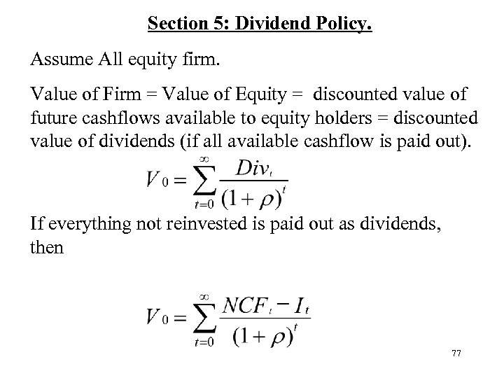Section 5: Dividend Policy. Assume All equity firm. Value of Firm = Value of Equity = discounted value of future cashflows available to equity holders = discounted value of dividends (if all available cashflow is paid out). If everything not reinvested is paid out as dividends, then 77

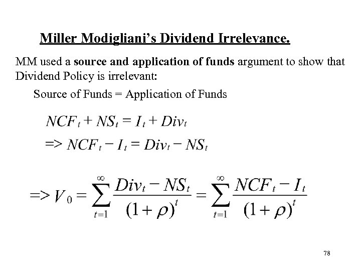Miller Modigliani’s Dividend Irrelevance. MM used a source and application of funds argument to show that Dividend Policy is irrelevant: Source of Funds = Application of Funds 78

-Dividends do not appear in the equation. -If the firm pays out too much dividend, it issues new equity to be able to reinvest. If it pays out too little dividend, it can use the balance to repurchase shares. -Hence, dividend policy irrelevant. -Key is the availability of finance in the capital market. 79

Example of Dividend Irrelevance using Source and Application of Funds. Firm invests in project giving it NCF = 100 every year, and it needs to re-invest, I =50 every year. Cashflow available to shareholders = NCF – I = 50. Now, NCF – I = Div – NS = 50. If firm pays dividend of 50, NS = 0 (ie it pays out exactly the cashflow available – no new shares bought or sold). If firm pays dividend of 80, NS = -30 (ie it sells new shares of 30 to cover dividend). If firm pays dividend of 20, NS = 30 (ie it uses cashflow not paid out as dividend to buy new shares). In each case, Div – NS = 50. 80

Gordon Growth Model. Where does growth come from? - retaining cashflow to re-invest. Constant fraction, K, of earnings retained for reinvestment. Rest paid out as dividend. Average rate of return on equity = r. Growth rate in cashflows (and dividends) is g = Kr. 81

Example of Gordon Growth Model. How do we use this past data for valuation? 82

Gordon Growth Model (Infinite Constant Growth Model). Let 83

Finite Supernormal Growth. -Rate of return on Investment > market required return for T years. -After that, Rate of Return on Investment = Market required return. If T = 0, V = Value of assets in place (re-investment at zero NPV). Same if r = 84

Examples of Finite Supernormal Growth. T = 10 years. K = 0. 1. A. Rate of return, r = 12% for 10 years, then 10% thereafter. B. B. Rate of return, r = 5% for 10 years, then 10% thereafter. 85

Are Dividends Irrelevant? - Evidence: higher dividends => higher value. - Dividend irrelevance : freely available capital for reinvestment. - If too much dividend, firm issued new shares. - If capital not freely available, dividend policy matter. Dividend Signalling - Miller and Rock (1985). NCF + NS = I + DIV: Source = Uses. DIV - NS = NCF - I. Right hand side = retained earnings. Left hand side - higher dividends can be covered by new shares. 86

Div - NS - E (Div - NS) = NCF - I - E (NCF - I) = NCF - E ( NCF). Unexpected dividend increase - favourable signal of NCF. E(Div - NS) = E(NCF - I) = 300. Date 1 Realisation: Firm B: Div - NS - E (Div - NS) = 500 = NCF - E ( NCF). Firm A : Div - NS - E (Div - NS) = -500 = NCF - E ( NCF). 87

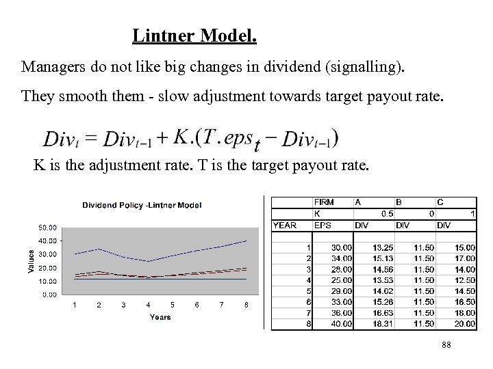Lintner Model. Managers do not like big changes in dividend (signalling). They smooth them - slow adjustment towards target payout rate. K is the adjustment rate. T is the target payout rate. 88

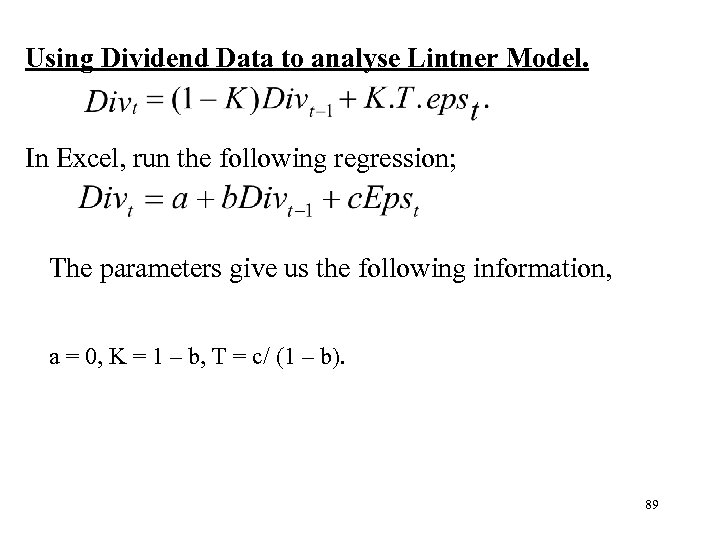Using Dividend Data to analyse Lintner Model. In Excel, run the following regression; The parameters give us the following information, a = 0, K = 1 – b, T = c/ (1 – b). 89

Comparison of MM Irrelevance, Gordon Growth, and Signalling. A. In MM irrelevance, Dividends do not matter: NCF – I is fixed each period. Dividends and NS balance out. Capital freely available. B. In Gordon Growth, NCF (1 -K) = NCF – I = Divs. No New shares. Increased Dividends => lower reinvestment, lower growth => effect on firm value? C. Signalling. High dividends => high firm value; low dividends => low firm value. (See Boyesen Case Study. ) 90

Section 6: Options and Risk Management. A call option gives the holder the right (but not the obligation) to buy shares at some time in the future at an exercise price agreed now. A put option gives the holder the right (but not the obligation) to sell shares at some time in the future at an exercise price agreed now. European Option – Exercised only at maturity date. American Option – Can be exercised at any time up to maturity. For simplicity, we focus on European Options. 91

Factors Affecting Price of European Option (=c). -Underlying Stock Price S. -Exercise Price X. -Variance of of the returns of the underlying asset , -Time to maturity, T. The riskier the underlying returns, the greater the probability that the stock price will exceed the exercise price. The longer to maturity, the greater the probability that the stock price will exceed the exercise price. 92

Combining options, graphic presentation. Buying a Call Option. Selling a put option. Buying a Put Option. 93

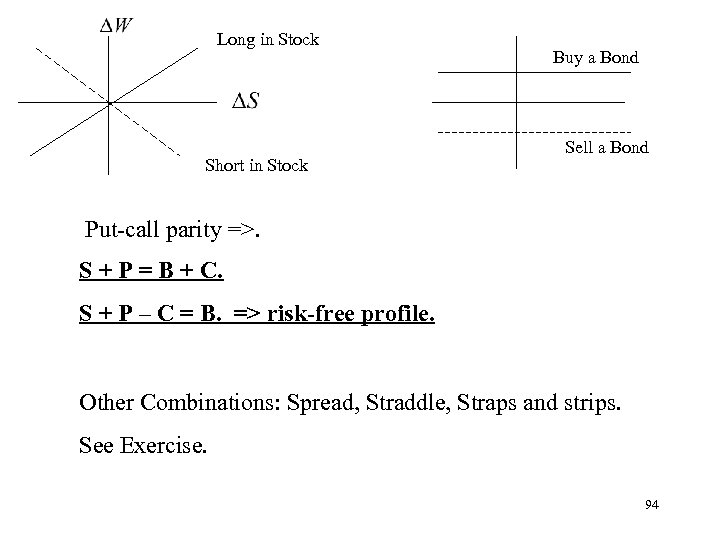Long in Stock Short in Stock Buy a Bond Sell a Bond Put-call parity =>. S + P = B + C. S + P – C = B. => risk-free profile. Other Combinations: Spread, Straddle, Straps and strips. See Exercise. 94

Options And Risk Management. Long in Stock Plus Sell a Call Option. +S S-C S + P – C = B. - C Plus buy a put: S + P – C = B. 95

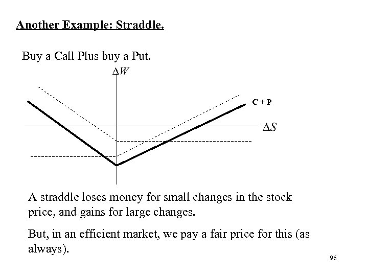Another Example: Straddle. Buy a Call Plus buy a Put. C+P A straddle loses money for small changes in the stock price, and gains for large changes. But, in an efficient market, we pay a fair price for this (as always). 96

Equity as a Call Option. Black and Scholes pointed out that equity is a call option on the value of the levered firm. If Value of firm exceeds face value of debt (exercise price of call option), equityholders pay the exercise price, and gain the increase in value. If value of firm is less than face value of debt, option is not exercised. Risky debt = risk-free debt – put option (B – P). 97

Important Implications for Firm. Equity is a call option: Value of Equity increases with risk. Value of Put option increases with risk: Therefore value of debt decreases with risk. After all, Equity holders have limited liability, and S = Max [ 0, V – D ]. B – P = Min [ V, D ]. With (B – P) + S = V. Therefore, if S increases, ( B – P) decreases. Equity holders will want to choose riskier projects. 98

Pricing Call Options – Binomial Approach. q u. S=24. 00 q c S=20 1 - q Cu = 3 d. S=13. 40 1 - q Cd=0 S = £ 20. q=0. 5. u=1. 2. d=. 67. X = £ 21. 1 + rf = 1. 1. Risk free hedge Portfolio: Buy One Share of Stock and write m call options. u. S - m. Cu = d. S – m. Cd => 24 – 3 m = 13. 40. ÞM = 3. 53. By holding one share of stock, and selling 3. 53 call options, your payoffs are the same in both states of nature (13. 40): Risk free. 99

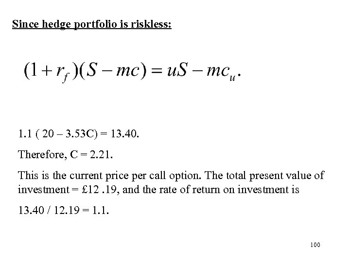Since hedge portfolio is riskless: 1. 1 ( 20 – 3. 53 C) = 13. 40. Therefore, C = 2. 21. This is the current price per call option. The total present value of investment = £ 12. 19, and the rate of return on investment is 13. 40 / 12. 19 = 1. 1. 100

Application of Options- Convertible Debt gives the holder the right (but not the obligation) to convert bonds into equity at a future date. Convertible debt is a combination of straight debt plus a call option. We saw that straight debt = risky debt – a put option. CD = D + C = B – P + C. Implication: Value of Convertible debt increases with risk of firm’s cashflows, and time to maturity. 101

Risk Management. Types of risk. -Interest rate risk. -exchange rate risk. -operating risks ÞIntegrated risk management approach. Two Main Questions: How do Managers engage in Risk Management? Should Managers even bother? 102

How to risk manage (Smith and Smithson). Use of derivatives. Interest rate, exchange rate instruments. Meulbroek- a) Modify firm’s operations b) Adjust capital structure c) Employ targeted financial Instruments. Need for an integrated risk management policy (explain? ) 103

Why bother risk-managing? (Meulbroek (2002), Shapiro and Titman Argument for risk-mgt irrelevance -A firm’s total risk consists of market risk (beta) and specific risk. -Well-diversified investors have already got rid of each firm’s specific risk. -Investors rewarded for holding market risk only (see CAPM). -Risk Management is at best irrelevant (cannot add value)- (like MM’s capital structure irrelevance). -At worst, a wasteful negative NPV activity (ie wasted resources, time and effort). 104

Argument for risk-management relevance (Meulbroek (2002), Shapiro and Titman Risk-management by firm is value-adding; - a) Inside info may make risk mgt easier for firms than investors. b) Financial distress. c) Non-diversified investors (such as managers themselves!!) d) Risk-mgt and management incentives (eg risk-shifting). e) Risk-mgt and debt capacity. 105

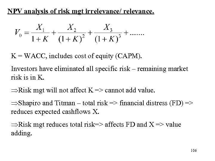NPV analysis of risk mgt irrelevance/ relevance. K = WACC, includes cost of equity (CAPM). Investors have eliminated all specific risk – remaining market risk is in K. ÞRisk mgt will not affect K => cannot add value. ÞShapiro and Titman – total risk => financial distress (FD) => reduces expected cashflows X. ÞRisk mgt reduces total risk=> affects FD and X => value adding. 106

Section 7: Convertible Debt. -Valuation of Convertibles. -Impact on Firm Value. -Why firms issue convertibles. -When are they converted (call policy)? Convertible bond -holder has the right to exchange the bond for common stock (equivalent to a call option). Conversion Ratio = number of shares received for each bond. Value of Convertible Bond = Max{ Straight bond value, 107 Conversion Value} +option value.

Value of Convertible Bond. (Occidental Electric Case Study) V Straight Bond Value Conversion Value Face Value Firm Value Total Value of Convertible Bond Firm Value 108

Conflict between Convertible Bond holders and managers. Convertible Bond = straight debt + call option. Value of a call option increases with: Time. Risk of firm’s cashflows. Implications: Holders of convertible debt maximise value by not converting until forced to do so => Managers will want to force conversion as soon as possible. Incentive for holders to choose risky projects => managers want to choose safe projects. 109

Reasons for Issuing Convertible Debt. Much real world confusion. Convertible debt - lower interest rates than straight debt. => cheap form of financing? No! Holders are prepared to accept a lower interest rate because of their conversion privilege. CD = 110

Alternative Analysis of Irrelevance of Convertible Debt. Firm Indifferent between issuing CD, debt or equity. -MM. 111

Why do firms issue convertible debt? If convertible debt is not a cheap form of financing, why is it issued? A. Equity through the Back Door (Stein, Mayers). -solves asymmetric information problems (see Myers-Majluf). -solves free cashflow problems. B. Convertible debt can solve risk-shifting problems. - If firm issues straight debt and equity, equity holders have an incentive to go for risky (value reducing) NPV projects. Since CD contains an option feature, CD value increases with risk. -prevents equity holders’ risk shifting. 112

Convertible Debt and Call Policy. Callable Convertible debt =>firms can force conversion. When the bond is called, the holder has 30 days to either: a) Convert the bond into common stock at the conversion ratio, or b) Surrender the bond for the call price. When should the bond be called? Option Theory: Shareholder wealth is maximised/ CD holders wealth is minimised if Firm calls the bond as soon as value = call price. 113

Call Puzzle. Manager should call the bond as soon as he can force conversion. Ingersoll (1977) examined the call policies of 124 firms 1968 -1975. - He found that companies delayed calling far too long. - median company waited until conversion value was 44% above call price - suboptimal. Call Puzzle addressed by Harris and Raviv. - signalling reasons for delaying calling. - early calling might signal bad news to the market. 114

Section 8: Takeovers. Merger Acquisition Stock Acquisition Takeovers Proxy Contest 1. Merger- must be approved by stockholders’ votes. 2. Stock acquisition- No shareholder meeting, no vote required. -bidder can deal directly with target’s shareholders- bypassing target’s management. - often hostile. -shareholders may holdout- freerider problems. 3. Proxy Contests- group of shareholders try to vote in new directors to the board. 115

Synergy = Example: Market Value after Merger. Firm A (bidder): cashflows = £ 10 m, r = 10%. = £ 100 m. Firm B (target): cashflows = £ 9 m, r = 15%. = £ 60 m. If A acquires B: Cashflows are expected to increase by £ 6 m P. A. Discount rate 20%. Synergy = £ 30 m. = $190 m. 116

The NPV of a merger. Firm A may have to pay a premium to acquire firm B. If firm A has to pay cost C to acquire firm B, NPV = Synergy - Premium. In our example, if C = 70, NPV of the merger to firm A = 30 - 10 = 20. Therefore, the gain from synergy can be divided between the bidder and the target - affected by the premium. (See Clifton Corporation Case Study). => models by Garvey and Hanka, and Grossman and Hart. 117

Garvey and Hanka: Management of Corporate Capital Structure. - Hostile takeovers, and US antitakeover laws of 1980’s. - dynamic defensive capital structure model. -Results- A. When takeover is easy => manager defends, increasing leverage => increases firm value => reduces takeover threat. B. When takeover is more difficult => manager reduces leverage to reduce financial distress. Optimal debt level maximises firm value. 118

- Manager’s optimal debt level minimises the threat of financial distress and minimises takeover threat. - Investors’ Optimal debt level D*, maximises firm value. - Firm has single terminal Cashflow: R + If no takeover threat, manager chooses D < R + - no financial distress. As takeover threat increases, manager increases D towards D* => V increases => reduces takeover threat. 119

Take-over Bids and the Freerider Problem (Grossman and Hart (----). - Market value per share under current management = Q. - Market value per share under optimal management = V. Price per share offered by raider = P, with Q < P V. Freerider problem - If shareholder accepts offer, he gets P. If shareholder refuses, but bid succeeds, he gets V. Therefore, all shareholders refuse - bid fails. Eg: Q = 10, V = 100. P = 20. Each shareholder will not tender for anything less than 100 raid fails. 120

Dilution - allows raider to take some of the firm’s value if successful. Eg: dilution = 10 (lump sum payment to raider). Successful raid: net value to shareholders = 100 - 10 = 90. Tender offer = 91. Bid succeeds. Implication of Garvey and Hanka, and Grossman and Hart. -Corporate Governance (disciplining) role of Takeovers. - Takeovers increase firm value (socially desirable). - Takeovers may be difficult to achieve due to defensive strategy, or freerider price ‘run-ups’. - Successful takeovers - most of the gains go to the target shareholders. 121

Effects of takeovers on stock prices of bidder and target. Successful Bids Unsuccessful Bids Jensen and Ruback JOFE 1983 122

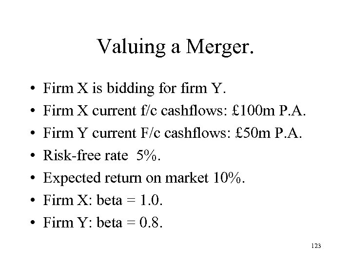Valuing a Merger. • • Firm X is bidding for firm Y. Firm X current f/c cashflows: £ 100 m P. A. Firm Y current F/c cashflows: £ 50 m P. A. Risk-free rate 5%. Expected return on market 10%. Firm X: beta = 1. 0. Firm Y: beta = 0. 8. 123

Post-merger. • • Combined company X + Y: beta = 1. 5 Combined cashflows X + Y: £ 300 m. What is synergy value? What is gain in shareholder wealth (for X and Y)? 124

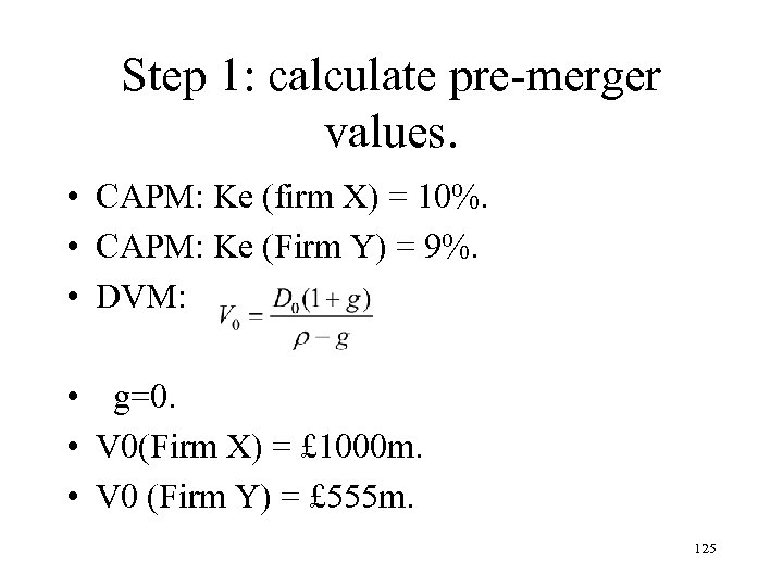Step 1: calculate pre-merger values. • CAPM: Ke (firm X) = 10%. • CAPM: Ke (Firm Y) = 9%. • DVM: • g=0. • V 0(Firm X) = £ 1000 m. • V 0 (Firm Y) = £ 555 m. 125

Step 2: Calculate post-merger value. • CAPM: Ke (A + B) = 12. 5% • V 0 (A + B) = £ 2400 m. • Synergy Value = 2400 – 1000 – 555 = 845 m (Total NPV of merger) • Which shareholders (X or Y) get this? 126

NPV of the Merger. X pays full value: C = 1400 => NPV X = 2400 – 1555 – 845 = 0. NPV Y = 1400 - 555 = 845. X pays pre-merger value: C = 555 => NPV X = 845. NPV Y = 555 – 555 = 0. 127

Which is most likely? • Free-rider problems. • Defensive use of capital structure. • Other defenses (poison pills; anti-takeover amendments etc). • Multiple bidders. • EMH. • Real Option approach. 128

Real Option Approach (AK). • • • Single Bidder X. Single Target Y. Bidder decides whether to make bid. Target decides whether to accept. Standard model: X just bids pre-bid value of Y. • AK model: options to delay for both X and Y. 129

Optimal bid. VY Pre. Y’s Minimum acceptable. VY Post. X’s Max bid 130