

605538a14649850a502755b18c2d73c9.ppt
- Количество слайдов: 42
 Monitoring and Modeling Managed Forest Ecosystems Using Interannual Multitemporal Landsat Data Randolph H. Wynne, Virginia Tech Buck Kline, Virginia Department of Forestry Christopher Potter, NASA Ames Christine Blinn, Susmita Sen, Valquiria Quirino, Patricia Donovan, Gene Yagow, and Carl Zipper, Virginia Tech Presented to Landsat Science Team June 2009
 Collective Achievements Ø Come together as a team Ø No-cost access to high quality data from full extent of US archive; activity on “repatriation” Ø Thermal back on Landsat 8 Ø OLI on time and within spec Ø Working toward Landsat 9 and beyond Ø Starting to think about products and associated preprocessing
 Key Points Ø Attribution of land cover change requires interannual multitemporal approach Ø Unmixing requires phenological information Ø There are important issues remaining with respect to both preprocessing and analysis of multitemporal data Ø Change in ecosystem structure and composition is insufficient; we need to be thinking about ecosystem function and associated services
 User Reported Primary Use of Landsat U. S. Users Only (Oct 1, 2008 – Mar 31, 2009)
 Delineate reclaimed coal mined areas of south western Virginia that have been mined and reclaimed in specific time periods within the study time frame (1984 -2008). Specific objectives: § Develop methods to separate reclaimed mines from other disturbances § Identify the year of mining for each mined pixel § Analyze the vegetation developmental pattern of each reclaimed mined pixel
 Study Area Coal mining counties of south west Virginia
 Data: 11 leaf-on Landsat TM images Path 18, Row 34 Landsat image dates 9/17/1984 6/6/1987 6/8/1988 9/21/1991 9/29/1994 9/5/1997 9/24/1998 6/9/2000 5/22/2002 6/2/2003 9/11/2005 Multi-temporal change detection Ø Identifying change using a series of 11 Landsat images from 1984 to 2005 Ø Detecting progressive change in landcover
 Spectral Trajectory Analysis Other Vegetation Indices tested: • NDMI • RSR • TC 1, 2 and 3 • DI Ideal spectral trajectory of a reclaimed mine
 Algorithm: Absolute drop and true slope • Find pixels with threshold drop • Identify the last year of visible mining • Find slope of recovery trajectory • Find lowest and highest NDVI
") Algorithm: Difference drop and difference slope • Identify pixels with difference drop (user defined) pe o Diff sl • Identify year of biggest drop • Determine slope of difference NDVI values in the recovery path (2 nd derivative of NDVI). • Find the max. decrease and the max. increase
Algorithm: Difference drop and difference slope • Identify pixels with difference drop (user defined) pe o Diff sl • Identify year of biggest drop • Determine slope of difference NDVI values in the recovery path (2 nd derivative of NDVI). • Find the max. decrease and the max. increase
 Reclaimed Mined Area Map • Year of mining: • Slope • Highest/lowest NDVI Year of mining Slope Highest/lowest NDVI
 Absolute drop and true slope output Input = stack of 11 NDVI images -0. 538 1 Lowest NDVI Year of mining OUTPUT Slope of recovery curve -0. 205 0. 189 Highest NDVI 0 1
 Results Level No. Mean Std Development 20 0. 03 0. 01 Mining Road 20 20 0. 06 0. 03 0. 01 Level No. Mean Std Development 20 0. 01 Mining 20 20 0. 05 0. 02 0. 01 Road
") Discussion Ø Sources of error in year mined output: i. ii. Roads (interstates/ highways) Urban developments Ø Source of error in slope: i. iii. iv. Year gap in time series Different seasonality of images Cloudy images Asymptotic nature of curve unaccounted in algorithm Ø Error caused by over classification of potentially disturbed lands. Ø Scale of fire and forest harvest insignificant with respect to mining.
Discussion Ø Sources of error in year mined output: i. ii. Roads (interstates/ highways) Urban developments Ø Source of error in slope: i. iii. iv. Year gap in time series Different seasonality of images Cloudy images Asymptotic nature of curve unaccounted in algorithm Ø Error caused by over classification of potentially disturbed lands. Ø Scale of fire and forest harvest insignificant with respect to mining.
 Forestry Reclamation Approach model of vegetative cover change over time. Four vegetation types are sown or planted during reclamation, but each type is dominant at a different stage. (Burger et al. , 2008)
 Graph showing NDVI values by landcover type throughout year. Reclaimed herbaceous fields have signature which is combination of pasture (dense, herbaceous vegetation) and bare soil signatures from early spring through summer.
 Powell River Site 2003 NAIP Forested SMA fraction
 Powell River Site 2005 NAIP Forested SMA fraction
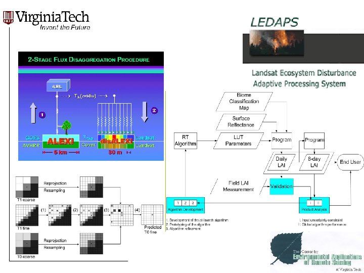
 22 image dates for Landsat 15/35 were processed through LEDAPS. 2) NDVI was") 1) 22 image dates for Landsat 15/35 were processed through LEDAPS. 2) NDVI was calculated on each SR and TOA image. 3) The mean NDVI for a forest stand of interest was calculated on all 44 images and plotted to compare the trend through time.
1) 22 image dates for Landsat 15/35 were processed through LEDAPS. 2) NDVI was calculated on each SR and TOA image. 3) The mean NDVI for a forest stand of interest was calculated on all 44 images and plotted to compare the trend through time.
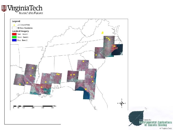
 LAI with Landsat 5 vs. Landsat 7 Site 175101 in Chatham, NC
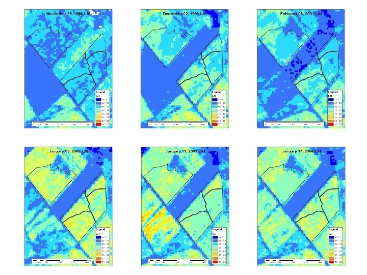
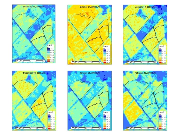
 Annual LAI Time Series for RW 194001 Based on Landsat TM Imagery Path 16 Row 36
 MODELS ESE · NASA-CASA GYC · PTAEDA 3. 1 · FASTLOB USDA Forest Service · FORCARB ESE MISSIONS · Aqua · Terra · Landsat 7 · ASTER Analysis Projects · IGBP-GCTE · IGBP-LUCC · USDA-FS FIA · USDA-FS FHM Decision Support for Forest Carbon Management: From Research to Operations DECISION SUPPORT: Current DSTs Information Products, Predictions, and Data from NASA ESE Missions: - MODAGAGG - MOD 12 Q 1 - MOD 13 - MOD 15 A 2 - ETM+ Level 1 WRS - AST L 1 B and 07 Linked DSTs and Common Prediction Framework (multiscale) • Growth • Yield • Product output • Ecosystem carbon pools • Partitioned NPP • NEP • Total C sequestration • Forecasts and scenarios Ancillary Data · SPOT · AVHRR NDVI · Forest inventory data · VEMAP climate data · SRTM topographic data Inputs • COLE (county-scale) • Lob. DST (stand-scale) • Growth and yield • Product output • Financial evaluations • CQUEST (1 km pixels) • Ecosystem carbon pools (g C/m 2) • Partitioned NPP (g C/m 2/yr) • NEP (g C/m 2/yr) Outputs Outcomes VALUE & BENEFITS Improve the rate of C sequestration in managed forests Decrease the cost of forest carbon monitoring and management Potentially slow the rate of atmospheric CO 2 increase Enhance forest soil quality Impacts
 Ø Remote Sensing for Forest Carbon Management Ø Regionwide CO 2 efflux and LAI acquired at network of monospecific sites with alternative forest management strategies Ø Landsat downscaling prototyped using STARFM; pine age class evaluation of algorithmic performance Ø Downscaled product being used for reducing variance in F S models across southeast (CASA, potentially Dis. ALEXI) Ø CASA modeling with Landsat done (FS, NEP) Ø Arc. GIS version of CASA complete Ø Fast. Lob C modifications made Ø CASA/Fast. Lob crosswalk in progress
 Modifications for Pine Growing Stands Landsat Reduced") NASA-CASA Ecosystem Model (Potter et al. 2007) Modifications for Pine Growing Stands Landsat Reduced Simple Ratio (monthly, 1 -km composites) Fertilizer N Landsat-based forest age mapping (0 -5, 6 -10, 11 -15, >15 year classes)
NASA-CASA Ecosystem Model (Potter et al. 2007) Modifications for Pine Growing Stands Landsat Reduced Simple Ratio (monthly, 1 -km composites) Fertilizer N Landsat-based forest age mapping (0 -5, 6 -10, 11 -15, >15 year classes)
 NASA-CASA model standing wood carbon in loblolly pine stands after 30 years of regrowth across the Virginia region. Units are in g C m-2 yr-1
 What Next? Ø Datasets obtained using industry cooperation have extensive long-term data on managed stands Ø Eddy flux for managed pines (2 age classes) in NC coastal plain Ø CASA-Fastlob crosswalk; web DSS Ø Broader ecosystem services framework

 Eco. Services Objective Ø To provide spatiallyexplicit, web-based quantification of ecosystem services using extant best of breed models at the tract level.
 Vision Ø Select tract via database or spatial query, enter other data as appropriate, and see bundled ecosystem services delivered Ø Real-time model runs rather than static scenarios Ø Alternative land use (1 st) and management (2 nd) options available for “what-if” scenarios Ø Innards model-independent, affording capacity to choose best-of-breed and facilitating updates to latest versions
 Initial Emphases
 Stand Output
 Biomass and Carbon Estimates Biomass estimates for the stem, branches, coarse roots, fine roots, first and second cohorts of foliage, and woody debris are added to the stand’s attribute table. Total above ground carbon estimates in Mg/Ha and Tons/Ac, stand acreage, and stand total above ground carbon in Mg and Tons are also added to the stand’s attribute table.
 Water Quality Ø Dr. Gene Yagow, VT BSE, program element lead Ø Current Chesapeake Bay program nutrient trading guidelines already implemented Ø Chesapeake Bay Watershed Model (CBWM) from EPA Chesapeake Bay Program selected ØCBWM based on Hydrologic Simulation Program. Fortran (HSPF) ØAll watersheds in Chesapeake Bay watershed states to be included in 2010 assessment
 Water Quality Ø Commonwealth of Virginia 305 b reporting through 2008 has used the Generalized Watershed Loading Functions (GWLF) model with 6 th order hydrologic units from the Nat’l Watershed Boundary Dataset Ø GWLF model calibrated to CBWM; all VA modeled Ø GWLF has some advantages for real-time simulation, including Ødaily vs. hourly (or shorter) time-steps Ørunoff and sediment loading factors
 Web Application
 Eco. Services Summary Ø Web-based credit calculators designed for use by land owners, land managers, and planners Ø Both land use (1 st) and land management (2 nd) scenarios supported Ø Focus on tract-level information Ø Bundled ecosystem services concept Ø Best-of-breed modular model approach Ø Field and remotely-sensed inputs
 Lessons for Team Ø Time series analysis opens up wonderful opportunities for land use and land cover change, but important research issues remain Ø Ecosystem function and resulting services as important as land use/cover, and requires a larger suite of products (LAI/f. PAR, VIs, etc. )
 Thanks! Randolph H. Wynne