Monetary Policy and Inflation Quantity Theory of Money

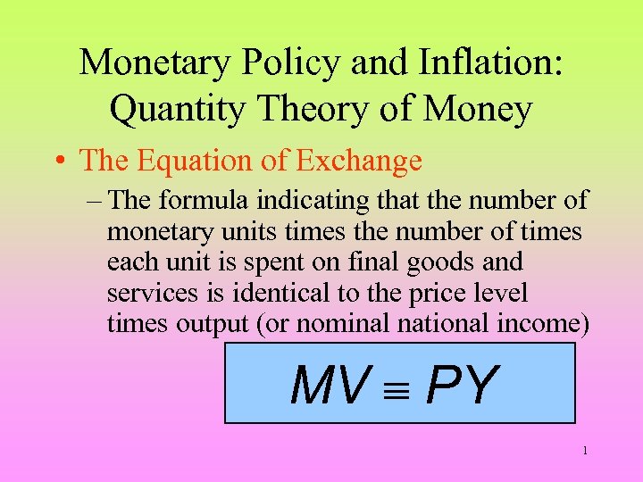Monetary Policy and Inflation: Quantity Theory of Money • The Equation of Exchange – The formula indicating that the number of monetary units times the number of times each unit is spent on final goods and services is identical to the price level times output (or nominal national income) MV º PY 1

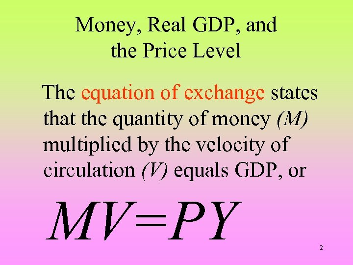Money, Real GDP, and the Price Level The equation of exchange states that the quantity of money (M) multiplied by the velocity of circulation (V) equals GDP, or MV=PY 2

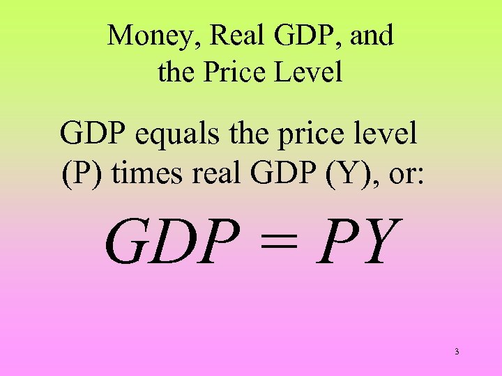Money, Real GDP, and the Price Level GDP equals the price level (P) times real GDP (Y), or: GDP = PY 3

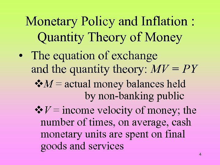Monetary Policy and Inflation : Quantity Theory of Money • The equation of exchange and the quantity theory: MV = PY v. M = actual money balances held by non-banking public v. V = income velocity of money; the number of times, on average, cash monetary units are spent on final goods and services 4

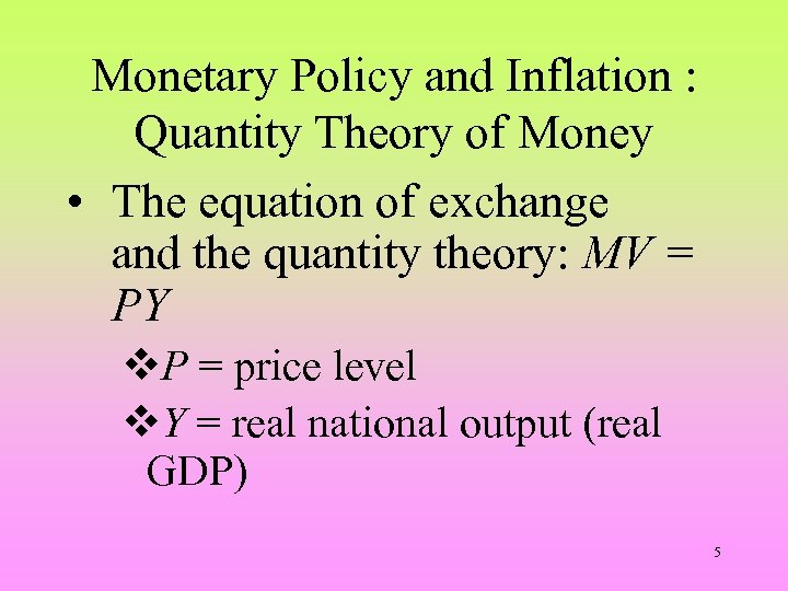Monetary Policy and Inflation : Quantity Theory of Money • The equation of exchange and the quantity theory: MV = PY v. P = price level v. Y = real national output (real GDP) 5

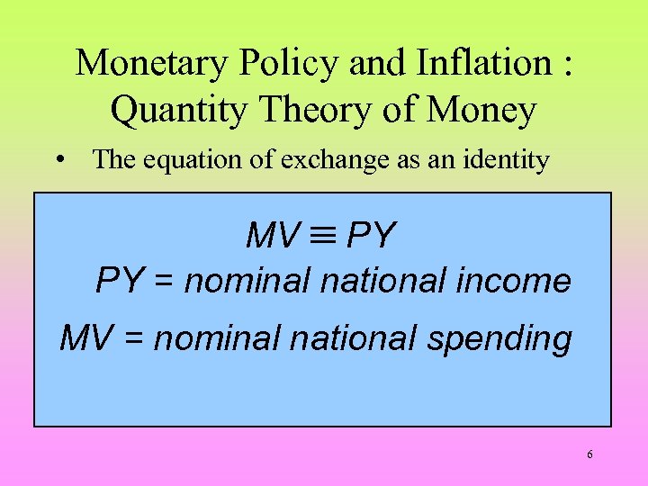Monetary Policy and Inflation : Quantity Theory of Money • The equation of exchange as an identity MV º PY PY = nominal national income MV = nominal national spending 6

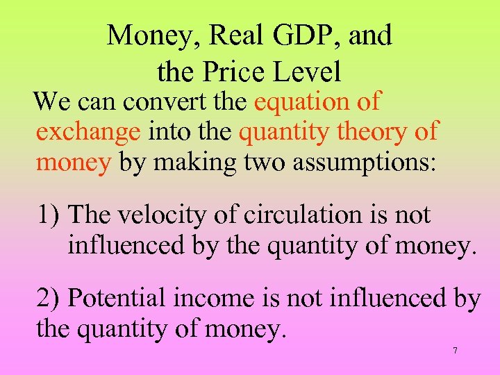Money, Real GDP, and the Price Level We can convert the equation of exchange into the quantity theory of money by making two assumptions: 1) The velocity of circulation is not influenced by the quantity of money. 2) Potential income is not influenced by the quantity of money. 7

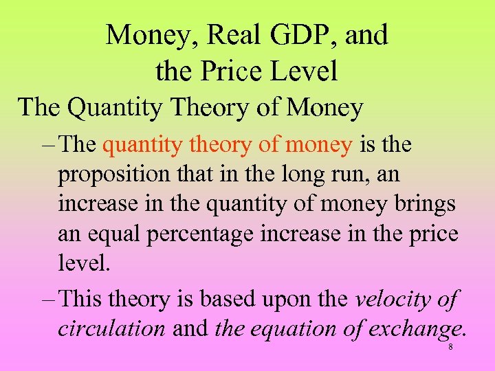Money, Real GDP, and the Price Level The Quantity Theory of Money – The quantity theory of money is the proposition that in the long run, an increase in the quantity of money brings an equal percentage increase in the price level. – This theory is based upon the velocity of circulation and the equation of exchange. 8

Money, Real GDP, and the Price Level The Quantity Theory of Money The velocity of circulation is the average number of times a dollar of money is used annually to buy goods and services that make up GDP. 9

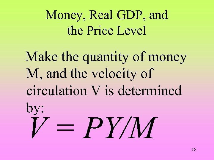Money, Real GDP, and the Price Level Make the quantity of money M, and the velocity of circulation V is determined by: V = PY/M 10

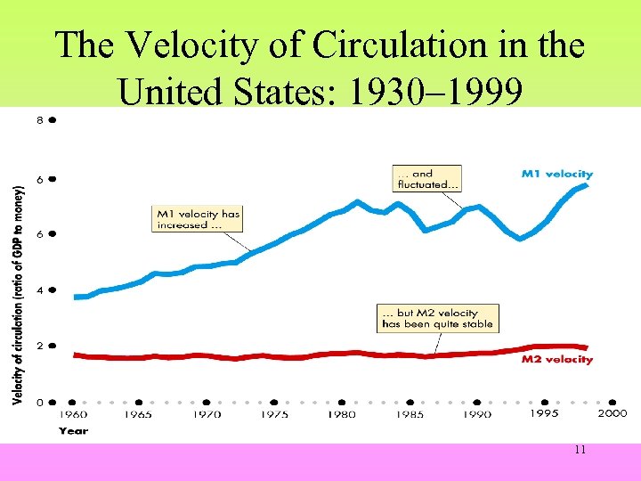The Velocity of Circulation in the United States: 1930– 1999 11

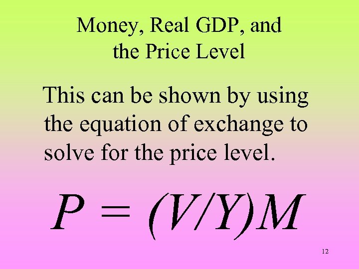Money, Real GDP, and the Price Level This can be shown by using the equation of exchange to solve for the price level. P = (V/Y)M 12

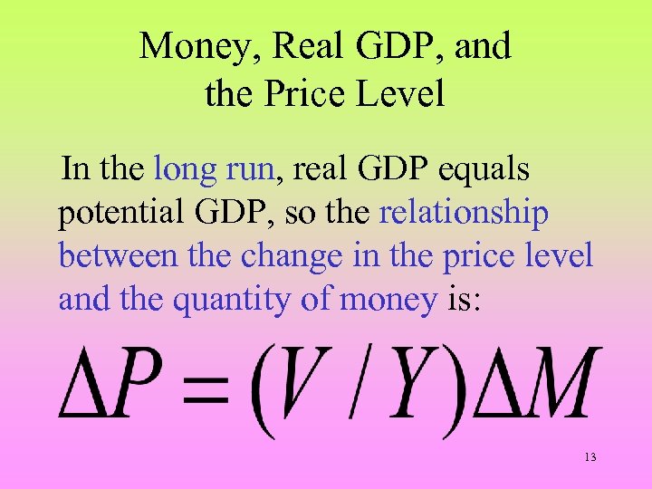Money, Real GDP, and the Price Level In the long run, real GDP equals potential GDP, so the relationship between the change in the price level and the quantity of money is: 13

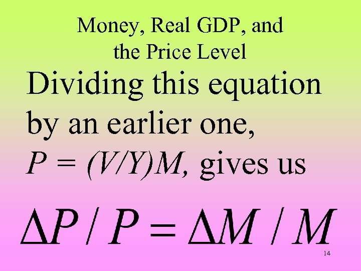Money, Real GDP, and the Price Level Dividing this equation by an earlier one, P = (V/Y)M, gives us 14

Money, Real GDP, and the Price Level This equation shows that the proportionate change in the price level equals the proportionate change in the quantity of money. This gives us the quantity theory of money: In the long run, the percentage increase in the price level equals the percentage increase in the quantity of money. 15

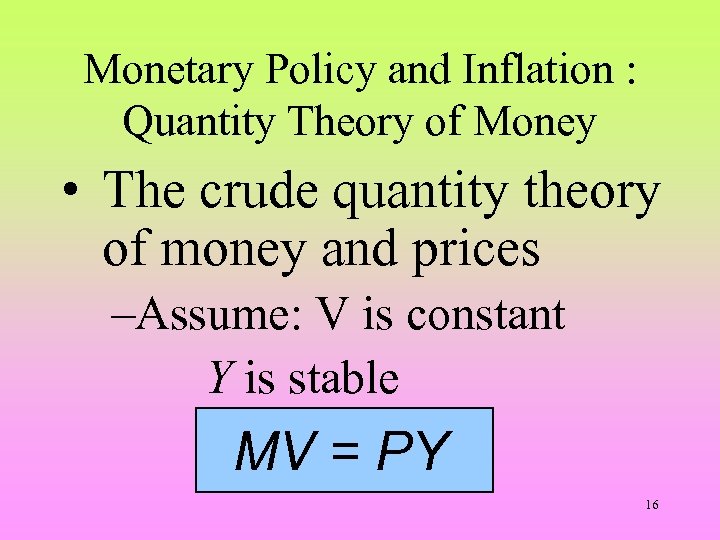Monetary Policy and Inflation : Quantity Theory of Money • The crude quantity theory of money and prices –Assume: V is constant Y is stable MV = PY 16

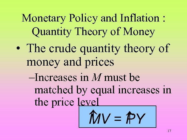Monetary Policy and Inflation : Quantity Theory of Money • The crude quantity theory of money and prices –Increases in M must be matched by equal increases in the price level M V = Y P 17

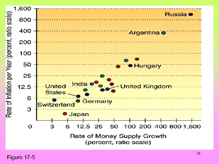Figure 17 -5 18

Money Growth and Inflation in the United States 19

Money Growth and Inflation in the United States 20

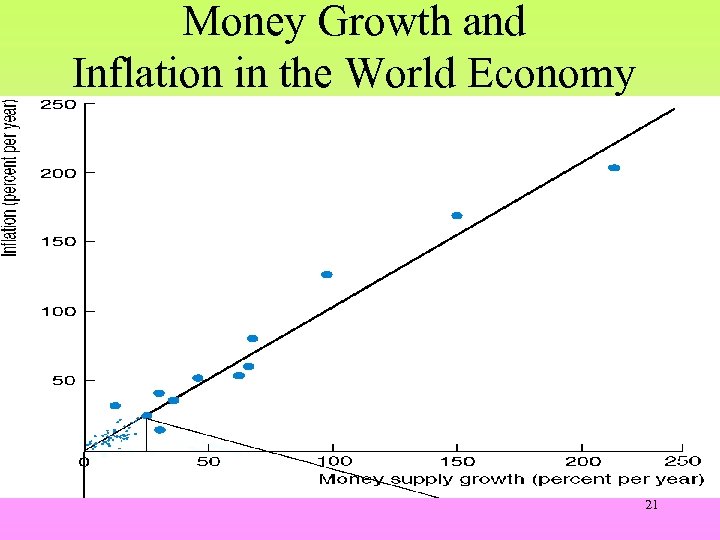Money Growth and Inflation in the World Economy 21

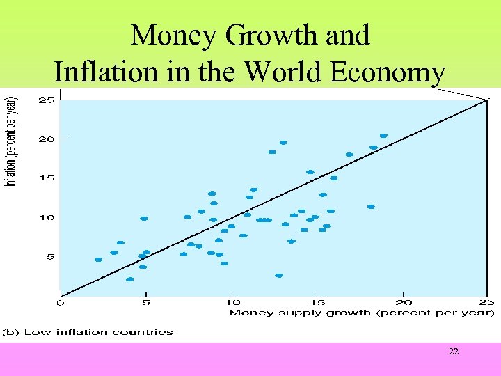Money Growth and Inflation in the World Economy 22

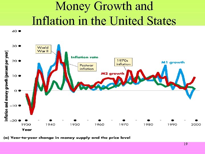
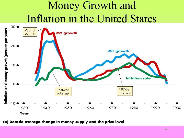
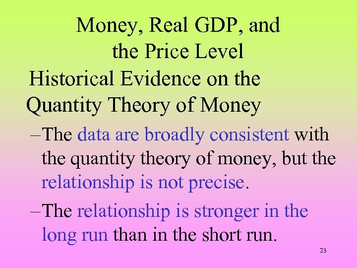Money, Real GDP, and the Price Level Historical Evidence on the Quantity Theory of Money – The data are broadly consistent with the quantity theory of money, but the relationship is not precise. – The relationship is stronger in the long run than in the short run. 23

Money, Real GDP, and the Price Level Correlation, Causation, and Other Influences The evidence shows that money growth and inflation are correlated. 24

Money, Real GDP, and the Price Level Correlation, Causation, and Other Influences This does not represent causation. • Does money growth cause inflation, or does inflation cause money growth? • Does some other factor cause inflation (deficit spending)? 25

Monetary Policy • The ultimate goal of all macro policy is to stabilize the economy at its fullemployment capacity. • A government has three basic tools of monetary policy: –Reserve requirements –Open-market operations –Discount rates 27

The Tools of Monetary Policy • Changes in the reserve requirements – An increase in the required reserve ratio • Makes it more expensive for banks to meet reserve requirements • Reduces bank lending – A decrease in the required reserve ratio • Makes it more expensive for banks to meet reserve requirements • Increases bank lending 28

Reserve Requirements • A lower reserve requirement increases the size of the money multiplier. – The money multiplier is the number of deposit (loan) dollars that the banking system can create from $1 of excess reserves. 29

A Decrease in Required Reserves • A change in the reserve requirement causes: – A change in excess reserves. – A change in the money multiplier. 30

The Impact of Reduced Reserve Requirement 31

The Monetary Base • The government can control the monetary base which equals –currency in public circulation plus bank reserves. 32

The Monetary Base • However, HKMA cannot control the amount of the monetary base that flows outside the country. 33

The Tools of Monetary Policy • Open market operations –The HKMA changes reserves by buying and selling bonds. 34

Open Market Activity • The HKMA purchases and sells government bonds to alter bank reserves. – By buying bonds — HKMA increases bank reserves. – By selling bonds — HKMA reduces bank reserves. 35

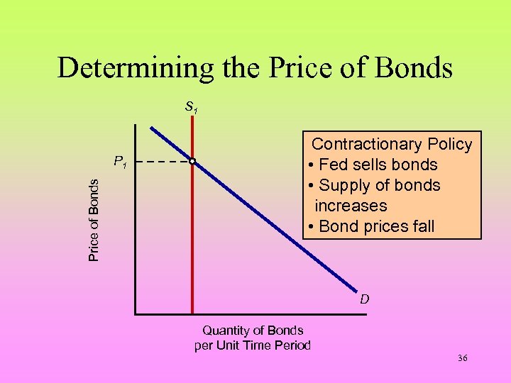Determining the Price of Bonds S 1 Price of Bonds P 1 Contractionary Policy • Fed sells bonds • Supply of bonds increases • Bond prices fall D Quantity of Bonds per Unit Time Period 36

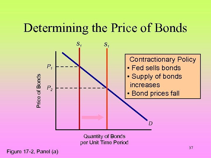Determining the Price of Bonds S 1 Price of Bonds P 1 P 2 S 1 Contractionary Policy • Fed sells bonds • Supply of bonds increases • Bond prices fall D Quantity of Bonds per Unit Time Period Figure 17 -2, Panel (a) 37

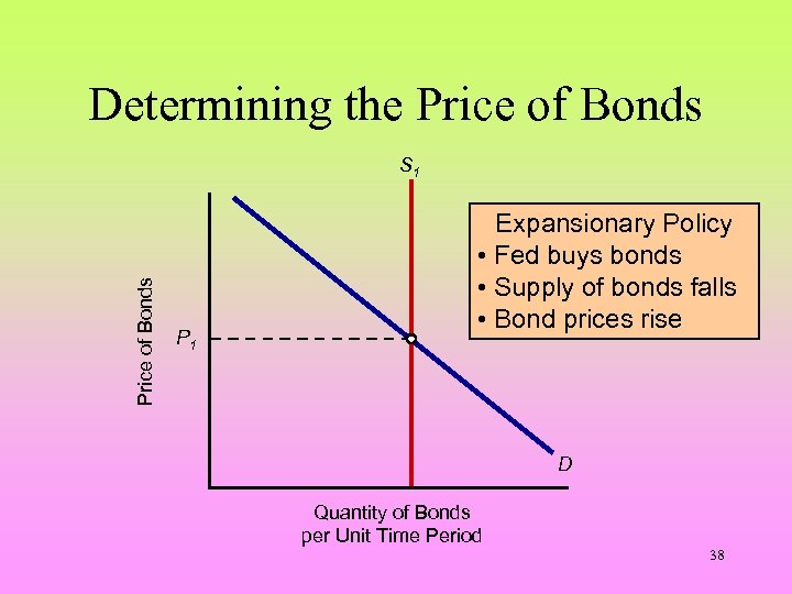Determining the Price of Bonds S 1 P 1 Expansionary Policy • Fed buys bonds • Supply of bonds falls • Bond prices rise D Quantity of Bonds per Unit Time Period 38

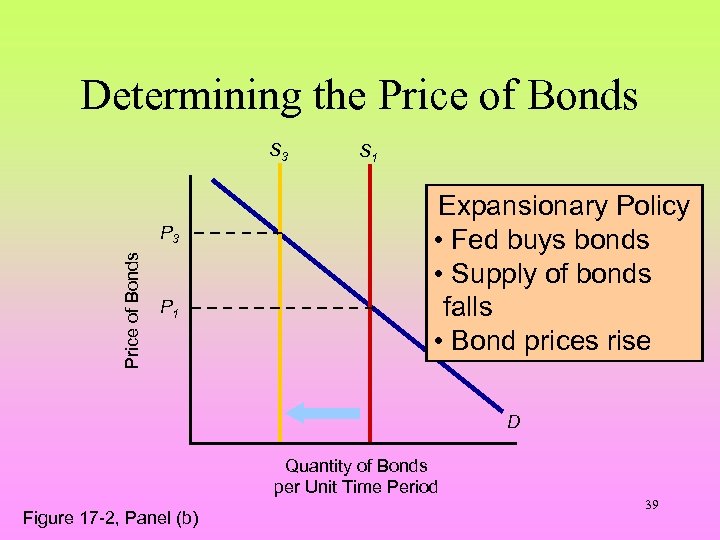Determining the Price of Bonds S 3 Price of Bonds P 3 P 1 S 1 Expansionary Policy • Fed buys bonds • Supply of bonds falls • Bond prices rise D Quantity of Bonds per Unit Time Period Figure 17 -2, Panel (b) 39

The Tools of Monetary Policy • Relationship between the price of existing bonds and the rate of interest – What happens to the interest on a bond when the price of a bond increases? 40

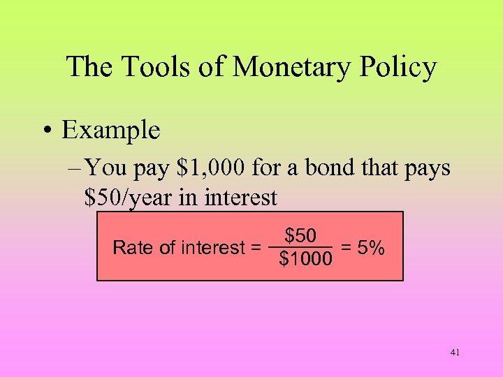The Tools of Monetary Policy • Example – You pay $1, 000 for a bond that pays $50/year in interest $50 Rate of interest = = 5% $1000 41

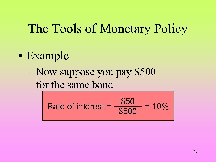The Tools of Monetary Policy • Example – Now suppose you pay $500 for the same bond $50 Rate of interest = = 10% $500 42

The Tools of Monetary Policy • The market price of existing bonds (and all fixed-income assets) is inversely related to the rate of interest prevailing in the economy. 43

The Tools of Monetary Policy • Changes in the discount rate - Increasing the discount rate increases the cost of borrowed funds for depository institutions that borrow reserves - Decreasing the discount rate decreases the cost of borrowed funds for depository institutions that borrow reserves 44

Effects of an Increase in the Money Supply • When the money supply increases people have too much money –How can this be? –Have you ever had too much money? 45

Effects of an Increase in the Money Supply • If you have a savings account the answer is “yes. ” • We must distinguish between income and money 46

Tools of Monetary Policy • Expansionary monetary policy: effects on aggregate demand, the price level, and real GDP • Monetary policy can be used to move the economy to its fullemployment potential. 47

Monetary Policy During Periods of Underutilized Resources • Monetary policy can generate increases in the equilibrium level of real GDP. 48

Expansionary Policy • The HKMA can increase AD/AE by increasing the money supply by: – Lowering reserve requirements. – Dropping the discount rate. – Buying more bonds: it increases bank lending capacity. 49

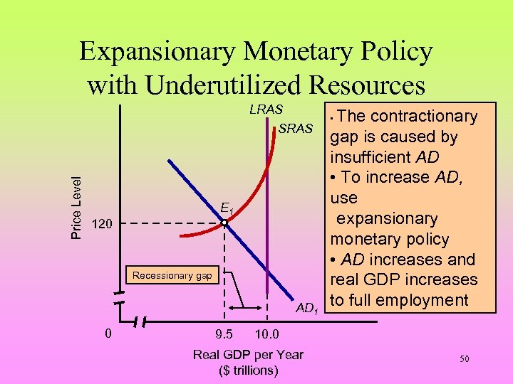Expansionary Monetary Policy with Underutilized Resources LRAS Price Level SRAS E 1 120 Recessionary gap AD 1 0 9. 5 The contractionary gap is caused by insufficient AD • To increase AD, use expansionary monetary policy • AD increases and real GDP increases to full employment • 10. 0 Real GDP per Year ($ trillions) 50

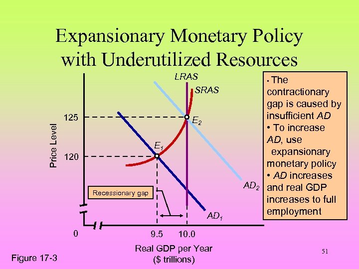Expansionary Monetary Policy with Underutilized Resources LRAS • The SRAS Price Level 125 E 2 E 1 120 AD 2 Recessionary gap AD 1 0 Figure 17 -3 9. 5 contractionary gap is caused by insufficient AD • To increase AD, use expansionary monetary policy • AD increases and real GDP increases to full employment 10. 0 Real GDP per Year ($ trillions) 51

Exhibit 4: Expansionary Monetary Policy to Correct a Contractionary Gap 52

Open Economy Transmission of Monetary Policy • The net export effect – Impact of expansionary monetary policy • increase the money supply • interest rates fall • value of the local currency falls • net exports increase • the net export effect complements the effectiveness of monetary policy by making greater income growth 53

Open Economy Transmission of Monetary Policy • The net export effect – Impact of expansionary fiscal policy revisited • • • larger deficit higher interest rates attracts foreign capital value of the local currency appreciates net exports fall net export effect reduces the effectiveness of fiscal policy by making smaller income growth 54

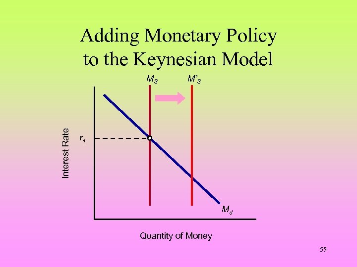Adding Monetary Policy to the Keynesian Model Interest Rate MS M’S r 1 Md Quantity of Money 55

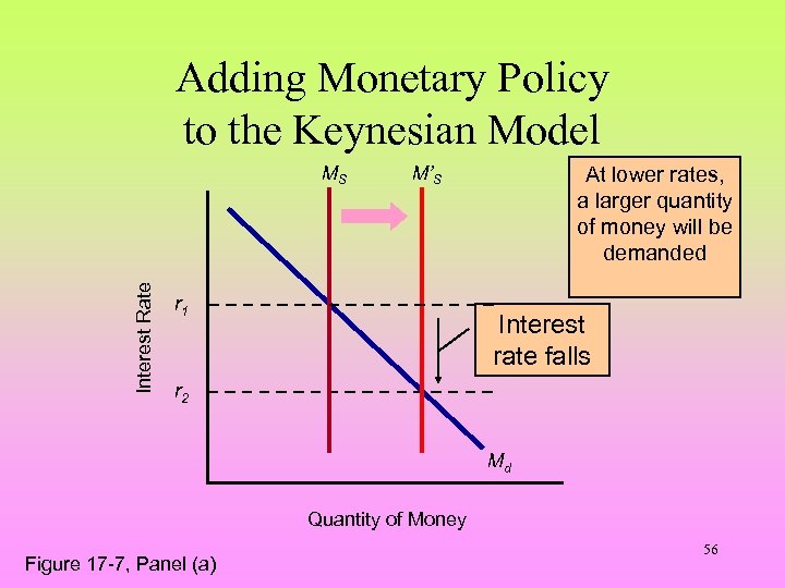Adding Monetary Policy to the Keynesian Model Interest Rate MS M’S r 1 At lower rates, a larger quantity of money will be demanded Interest rate falls r 2 Md Quantity of Money Figure 17 -7, Panel (a) 56

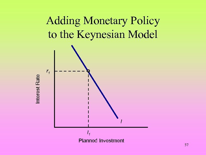Interest Rate Adding Monetary Policy to the Keynesian Model r 1 I I 1 Planned Investment 57

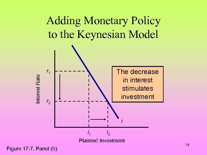Interest Rate Adding Monetary Policy to the Keynesian Model The decrease in interest stimulates investment r 1 r 2 I I 1 I 2 Planned Investment Figure 17 -7, Panel (b) 58

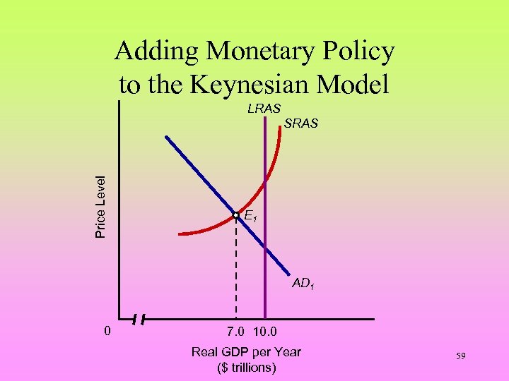Adding Monetary Policy to the Keynesian Model LRAS Price Level SRAS E 1 AD 1 0 7. 0 10. 0 Real GDP per Year ($ trillions) 59

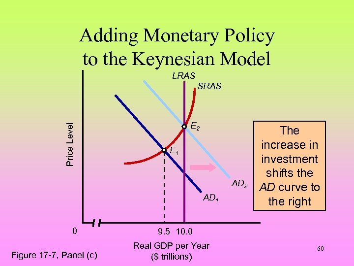Adding Monetary Policy to the Keynesian Model LRAS Price Level SRAS E 2 E 1 AD 2 AD 1 0 Figure 17 -7, Panel (c) The increase in investment shifts the AD curve to the right 9. 5 10. 0 Real GDP per Year ($ trillions) 60

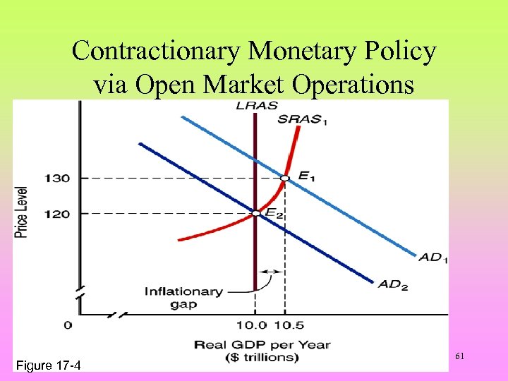Contractionary Monetary Policy via Open Market Operations Figure 17 -4 61

Monetary Policy in Action: The Transmission Mechanism • The monetarist’s views of money supply changes – They are those Macroeconomists who believe that inflation is always caused by excessive monetary growth and that changes in the money supply affect AD both directly and indirectly 62

Monetary Policy in Action: The Transmission Mechanism • The monetarist’s views of money supply changes – Increase in the money supply increases aggregate demand directly – Based on the equation of exchange, prices always rise when the money supply is increased 63

Monetary Policy in Action: The Transmission Mechanism • Monetarists’ criticism of monetary policy – Time lags are too long to use monetary policy effectively – Monetary policy is seen as a destabilizing force 64

Monetary Policy in Action: The Transmission Mechanism • Monetary Rule – A monetary policy that incorporates a rule specifying the annual rate of growth of some monetary aggregate – Example • Increase in the money supply smoothly at a rate consistent with the economy’s long-run average growth rate measured in terms of NI % change 65

Monetary Policy in Action: The Transmission Mechanism • What do you think? –What would happen to the effectiveness of the monetary rule if V is not stable? 66

Price vs. Output Effects • The success of monetary policy depends on the conditions of aggregate demand aggregate supply. 67

Aggregate Supply • The shape of the AS curve determines the effectiveness of expansionary monetary policy in raising output. 68

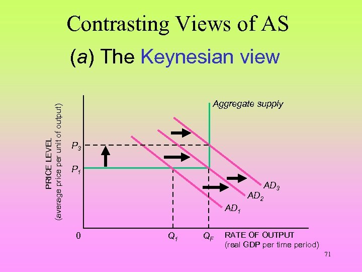
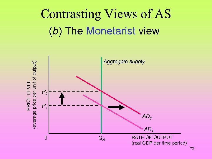
Aggregate Supply • Horizontal AS — output increases without any inflation/price change. • Vertical AS — inflation occurs without changing output. • Upward sloping AS — both prices and output are affected by monetary policy. 69

Aggregate Supply • With an upward-sloping AS curve, expansionary policy causes some inflation and restrictive policy causes some unemployment. 70

Contrasting Views of AS PRICE LEVEL (average price per unit of output) (a) The Keynesian view Aggregate supply P 3 P 1 AD 2 AD 3 AD 1 0 Q 1 QF RATE OF OUTPUT (real GDP per time period) 71

Contrasting Views of AS PRICE LEVEL (average price per unit of output) (b) The Monetarist view Aggregate supply P 5 P 4 AD 5 AD 4 0 QN RATE OF OUTPUT (real GDP per time period) 72

Figure 28 -10 Two Views on the Strength of Monetary Changes 73

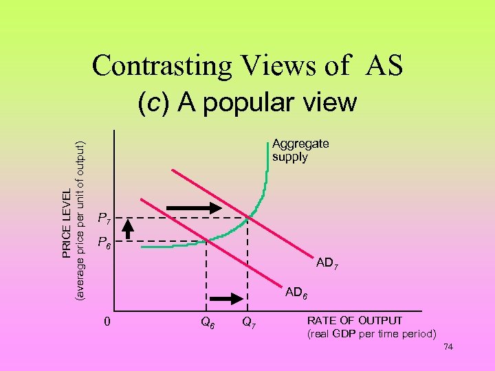Contrasting Views of AS PRICE LEVEL (average price per unit of output) (c) A popular view Aggregate supply P 7 P 6 AD 7 AD 6 0 Q 6 Q 7 RATE OF OUTPUT (real GDP per time period) 74

Policy Perspectives • The shape of the aggregate supply curve spotlights a central policy debate. 75

Fixed Rules or Discretion? • Should the government try to fine-tune the economy with constant adjustments of the money supply? 76

Fixed Rules or Discretion? • Or should the government instead simply keep the money supply growing at a steady pace? 77

Discretionary Policy • The economy is constantly beset by expansionary and recessionary forces. • There is a need for continual adjustments to money supply. 78

Fixed Rules • Critics of discretionary monetary policy raise objections linked to the shape of the AS curve. • AS curve could be vertical or at least upward sloping. 79

Fixed Rules • With an upward-sloping AS curve, too much expansionary monetary policy leads to inflation. 80

Fixed Rules • Fixed rules for moneysupply management are less prone to error than discretionary policy. 81

Fixed Rules • The money supply should increase by a constant (fixed) rate each year equal to that of potential Y growth. 82