Modern problems in the Artic Ocean modeling Nikolay

Modern problems in the Artic Ocean modeling Nikolay [YI]akovlev INM RAS, Moscow, Russia Joint INM – Hamburg University seminar on modern problems in atmosphere-ocean modeling Moscow, 18 June 2010.

1. INM RAS efforts in Arctic Ocean modeling. 2. Some problems with the ice and ocean numerical model formulations. 3. Some considerations on the explicit treatment of tides in AO models. N. Yakovlev, INM RAS, Moscow

The global version of the model is used as the oceanic component of the IPCC climate model INMCM 3 which is presented in the IPCC Fourth Assessment Report (2007). INM RAS eddy-permitting ocean circulation σ-model The present version of the model is realized for coupled North Atlantic (open boundary at 20°S) - Arctic Ocean – Bering Sea region including Mediterranean and Black Seas. A rotation of the model grid is employed in order to avoid the problem of converging meridians over the Arctic ocean. The model North Pole is located at geographical equator, 120°W. 1/4° horizontal eddy-permitting resolution is used (620 x 440 grid points) and 27 unevenly spaced vertical levels. Biharmonic operator is used for lateral viscosity and Monin-Obuhov-Kochergin parameterization is used for vertical diffusion and viscosity. The EVP (elastic- viscous- plastic) dynamic thermodynamic sea ice model (Hunke, 2001; Iakovlev, 2005) is embedded. Model domain

The design of the experiment The numerical experiment was carried out using the realistic global atmosphere forcing for years from 1958 to 2006 provided by GFDL for CLIVAR Common Ocean -ice Reference Experiments (CORE). http: //data 1. gfdl. noaa. gov/nomads/forms/mom 4/CORE. html The heat, salt and momentum fluxes at the sea surface are calculated using 6 hr wind, pressure, temperature and humidity; daily shortwave and longwave radiation; monthly precipitation and year mean river runoff. Sensible and latent heat fluxes employ bulk formulas using CORE data and model SST. Restoring to observed sea surface salinity with coefficient of 1/(30 days) is used for salt flux. Time step: 1 hour. Initial conditions: Levitus data for temperature and salinity and no motion for velocity. Duration: 20 year spin-up, then realistic circulation for years 1958 - 2006.

Model ice concentration vs. observational data http: //nsidc. org/data/seaice_index/archives/image_select. html for High NAO index

Model ice concentration vs. observational data http: //nsidc. org/data/seaice_index/archives/image_select. html for Low NAO index

Velocity (top panels) and temperature (bottom panels) sections for West Spitsbergen (left) and Nord Cape (right) currents (mean for 1998 -2006 yrs). (latitude and longitude in model coordinates). Section 1 Section 2

INM RAS Model FEMAO-1 1. 3 D primitive ocean dynamics equations with free upper surface 2. EVP sea ice rheology 3. Ice thickness redistribution according to Hibler, 1980, Flato & Hibler, 1995 4. Forcing according to AOMIP protocol (ocean, rivers, atmosphere, salinity restoring time scale 180 days) 5. Low spatial resolution to develop local physics parameterizations (100 km) 6. Tide М 2, specified as boundary conditions (Norwegian Sea, Denmark Strait, Bering Strait, Canadian Archipelago passages) Flather, 1976. N. Yakovlev, INM RAS, Moscow

N. Yakovlev, INM RAS, Moscow

Fram Strait temperature salinity velocity N. Yakovlev, INM RAS, Moscow

Mean Ice drift velocity, cm/s ? N. Yakovlev, INM RAS, Moscow

Model, December 1993 7. 22 см/s Satellite Data, December 1993 ~ 8 см/s Satellite Data From: ftp: //ftp. ifremer. fr/ifremer/cersat/products/gridded/psidrift/data/arctic/) N. Yakovlev, INM RAS, Moscow

Model, February 1994 3. 25 см/s Satellite Data, February 1994 ~ 3 см/s Satellite Data From: ftp: //ftp. ifremer. fr/ifremer/cersat/products/gridded/psidrift/data/arctic/) N. Yakovlev, INM RAS, Moscow

Sea Ice

Second-generation Louvain-la-Neuve Ice-ocean Model (SLIM)

Ocean

Model Design 1. Various vertical coordinates free surface z-model Partial step topography • Trivial pressure gradient errors • Decades of experience • Well known limitations • Irregular and variable computational domain (i. e. , land/sea masks and vanishing surface layer) • Terrain following σ-model • Smooth topography • Regular computational domain (no land/sea masks) • Time independent computational domain (-1 < sigma < 0) • Pressure gradient errors: requires topography filters • Difficult neutral physics implementation: not commonly done in sigma-models • Irregular computational domain (i. e. , land/sea masks needed) • Time independent computational domain (-H < z* < 0): no vanishing layers. • Negligible pressure gradient errors since isosurfaces are quasihorizontal. Correspondingly, can use the same neutral physics technology as in z-models. N. Yakovlev, INM RAS, Moscow

z/z*/p/p* ρ POSUM Hy. COM Poseidon HIM MIT z/z*/p/p*/ MOM POP σ ROMS σ POM N. Yakovlev, INM RAS, Moscow

2. Bottom topography approximation (partial cells and «shaved» cells) – errors in the pressure gradient approximation in the lowermost layer Not in the climate models! N. Yakovlev, INM RAS, Moscow

Quasi-Physical parameterizations: Cascading and Cross-Ridge Exchanges N. Yakovlev, INM RAS, Moscow

Tidal mixing n Tides provide about half of the energy for mixing in the open ocean. n At topography tidal energy is converted to waves (baroclinic tides) and/or mixing. n Waves eventually lead to mixing remote from generation site. n Effects of tides need to be included in climate simulations. N. Yakovlev, INM RAS, Moscow

Holloway, G. , and A. Proshutinsky (2007), Role of tides in Arctic ocean/ice climate, J. Geophys. Res. , 112, C 04 S 06, doi: 10. 1029/2006 JC 003643. Periodic changes and strong ice shear were observed by early northern travelers in the Barents and White Seas (Litke, 1844). Nansen (1898, 1902) reported the spring neap cycle of "ice pressure" affecting the Fram as it drifted with ice, and suggested that this was a result of ice interaction with the M 2 tidal wave propagating from the North Atlantic. The importance of tides in ice covered seas was corroborated by Sverdrup (1926), Zubov (1945), Murty (1985), Prinsenberg (1988), Bourke and Parsons (1993), Pease et al. (1994, 1995), and many others. The main conclusions: 1. Results clearly show enhanced loss of heat from Atlantic waters. 2. The impact of tides on sea ice is more subtle as thinning due to enhanced ocean heat flux competes with net ice growth during rapid openings and closings of tidal leads. N. Yakovlev, INM RAS, Moscow

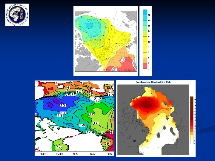
Tide Intensifies Vertical Mixing (the illustration to the conclusion above) Data by Kowalik & Proshutinsky, 1994 Kowalik, Z. , and A. Yu. Proshutinsky, 1994. The Arctic Ocean Tides, In: The Polar Oceans and Their Role in Shaping the Global Environment: Nansen Centennial Volume, Geoph. Monograph 85, AGU, 137 --158. N. Yakovlev, INM RAS, Moscow

The role of tides in the Arctic Ocean thermohaline structure formation Прошутинский А. Ю. Колебания уровня Северного Ледовитого океана. Санкт. Петербург. Гидрометеоиздат. 1993. 216 с. Kowalik, Z. , and A. Yu. Proshutinsky, 1995. Topographic enhancement of tidal motion in the western Barents Sea. J. Geophys. Res. , 100(C 2), 2613 -2637. Polyakov, I. , E. Dmitriev, and A. Proshutinsky, 1995. Modeling of a three-dimensional structure of the Arctic Ocean M_2 tide with a high spatial resolution. Cray Channels, 17(2), p. 36. N. Yakovlev, INM RAS, Moscow

M 2 Sea Level Amplitude (cm) Kowalik & Proshutinsky 1994 Kowalik, Z. , and A. Yu. Proshutinsky, 1994. The Arctic Ocean Tides, In: The Polar Oceans and Their Role in Shaping the Global Environment: Nansen Centennial Volume, Geoph. Monograph 85, AGU, 137 --158. INM RAS FEMAO-1 N. Yakovlev, INM RAS, Moscow

M 2 maximum velocity (cm/s) Kowalik & Proshutinsky 1994 INM RAS FEMAO-1 N. Yakovlev, INM RAS, Moscow

It is wrong approach just to «embed» tide into a general circulation model – the results may be any but the right ones. N. Yakovlev, INM RAS, Moscow

N. Yakovlev, INM RAS, Moscow

The parameterizations of the ice-ocean drag «Levitating» ice (ice as a flat rigid plate) Parameterization with «hummocking» of ice (Standard Russian textbook: Доронин Ю. П. Динамика океана, 1980) Non-stratified ocean: M. STEELE, J. H. MORISON, AND N. UNTERSTE 1 NER. The Partition of Air-Ice-Ocean Momentum Exchange as a Function of Ice Concentration, Floe Size, and Draft. JGR, V. 94, NO. C 9, P. 12, 739 -12, 750, 1989. Stratified ocean, Ice cover with regular spatial strucuture: M. G. MCPHEE, L. H. KANTHA. Generation of Internal Waves by Sea Ice. JGR, V. 94, NO. C 3, P. 3287 -3302, 1989. N. Yakovlev, INM RAS, Moscow

Lab Experimental Data Pite, D. H. , D. R. Topham and B. J. van Hardenberg. , 1995: Laboratory measurements of the drag force on a family of two-dimensional ice keel models in a two-layer flow, J. Phys. Oceanogr. , v. 25, 3008 -3031. Solid line – Stratified Ocean, dashed line – homogeneous ocean N. Yakovlev, INM RAS, Moscow

New Parameterization The main goal is to take into account seasonal variations of ice and ocean GWD: Miles, J. W. , 1969: Waves and wave drag in stratified flows. Proc. 12 th Inst. Congress of Applied mechanics, M. Hatenyi and W. G. Vincenti, Eds. , Springer-Verlag, 52 -76. Phillips, D. , 1984: Analytic surface pressure and drag for linear hydrostatic flow over threedimensional elliptic mountains. J. Atmos. Sci. , v. 41, 1073 -1084. Smith, R. B. , 1989: Hydrostatic airflow over mountains. Advances in Geophysics, v. 31, Academic Press, 1 -41. M. G. MCPHEE, L. H. KANTHA. Generation of Internal Waves by Sea Ice. JGR, V. 94, NO. C 3, P. 3287 -3302, 1989. Blocked Flow: Lott, F. and Miller, M. J. A new subgrid-scale orographic drag parameterization: Its formulation and testing. Q. J. R. Meteorol. Soc. V. 123, p. 101 -127, 1997. Wake effect: M. STEELE, J. H. MORISON, AND N. UNTERSTE 1 NER. The Partition of Air-Ice-Ocean Momentum Exchange as a Function of Ice Concentration, Floe Size, and Draft. JGR, V. 94, NO. C 9, P. 12, 739 -12, 750, 1989. N. Yakovlev, INM RAS, Moscow

GWD Blocked Flow N. Yakovlev, INM RAS, Moscow

SUMMARY 1. Modern models of the Arctic Ocean are quite skilled to reproduce many of the observed features of ice and ocean. 2. There are both numerical and physical problems in more detailed simulation of the AO. New numerical technologies should be accompanied by the new physical formulations. 3. The explicit simulation of tides should be accompanied by the revision of the parameterizations used in the model. It is necessary to take into account mechanisms, associated with the internal tides generation and with the singularities at the critical latitude 75 N.

The End