d1c98d3a61743857b2b869bc93c6335e.ppt
- Количество слайдов: 27
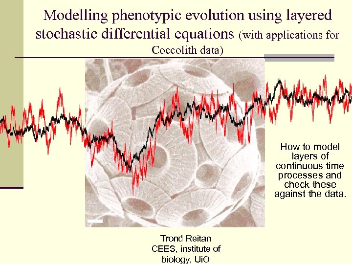 Modelling phenotypic evolution using layered stochastic differential equations (with applications for Coccolith data) How to model layers of continuous time processes and check these against the data. Trond Reitan CEES, institute of biology, Ui. O
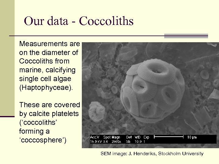 Our data - Coccoliths Measurements are on the diameter of Coccoliths from marine, calcifying single cell algae (Haptophyceae). These are covered by calcite platelets (‘coccoliths’ forming a ‘coccosphere’) SEM image: J. Henderiks, Stockholm University
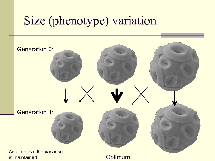 Size (phenotype) variation Generation 0: Generation 1: Assume that the variance is maintained Optimum
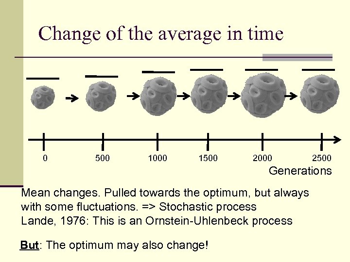 Change of the average in time 0 500 1000 1500 2000 2500 Generations Mean changes. Pulled towards the optimum, but always with some fluctuations. => Stochastic process Lande, 1976: This is an Ornstein-Uhlenbeck process But: The optimum may also change!
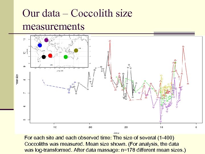 Our data – Coccolith size measurements For each site and each observed time: The size of several (1 -400) Coccoliths was measured. Mean size shown. (For analysis, the data was log-transformed. After data massage: n=178 different mean sizes. )
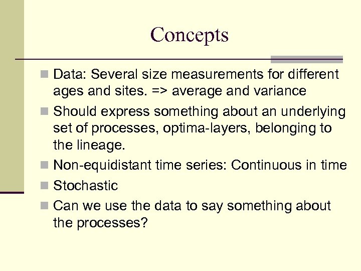 Concepts n Data: Several size measurements for different ages and sites. => average and variance n Should express something about an underlying set of processes, optima-layers, belonging to the lineage. n Non-equidistant time series: Continuous in time n Stochastic n Can we use the data to say something about the processes?
 Background n. Data: Jorijntje Henderiks. n. Tore Schweder: Idea and mathematical foundation. n. Me: Inference, programming and control calculations.
 Multiple layers of hidden processes – why? n Measured mean size is a noisy indicator of overall mean size at a given moment. n Even with perfect measurements, what happens between needs inference. n A phenotype character will track an evolutionary optimum (natural selection). n The optimum changes also. Can be further divided into layers describing global and local contributions. n Each layer is responding to what happens in a lower layer.
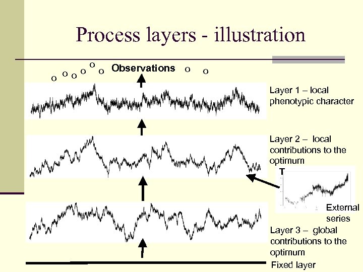 Process layers - illustration o o o Observations o o Layer 1 – local phenotypic character Layer 2 – local contributions to the optimum T External series Layer 3 – global contributions to the optimum Fixed layer
 Variants n Can have different number of layers. n In a single layer, one has the choice of: Ø Local or global parameters Ø The stochastic contribution can be global or local (sitespecific) Ø Correlation between sites (inter-regional correlation) Ø Deterministic response to the lower layer Ø Random walk (not responding to anything else, no tracking) n In total: 750 models examined
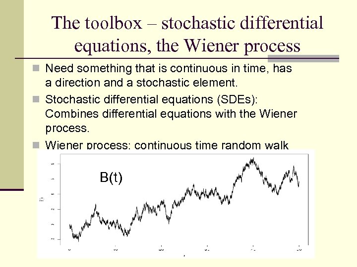 The toolbox – stochastic differential equations, the Wiener process n Need something that is continuous in time, has a direction and a stochastic element. n Stochastic differential equations (SDEs): Combines differential equations with the Wiener process. n Wiener process: continuous time random walk (Brownian motion). B(t)
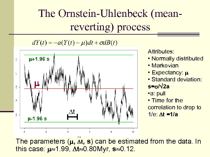 The Ornstein-Uhlenbeck (meanreverting) process 1. 96 s -1. 96 s t Attributes: • Normally distributed • Markovian • Expectancy: • Standard deviation: s= / 2 a • a: pull • Time for the correlation to drop to 1/e: t =1/a The parameters ( , t, s) can be estimated from the data. In this case: 1. 99, t 0. 80 Myr, s 0. 12.
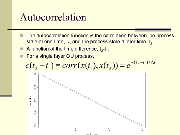 Autocorrelation n The autocorrelation function is the correlation between the process state at one time, t 1, and the process state a later time, t 2. n A function of the time difference, t 2 -t 1. n For a single layer OU process,
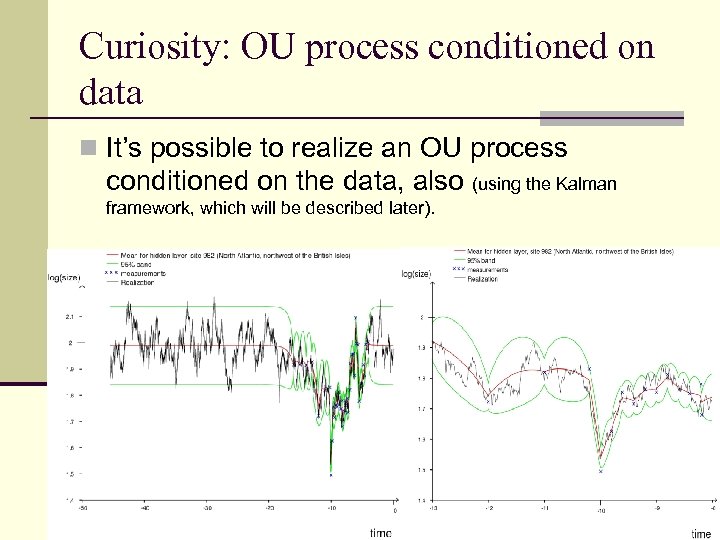 Curiosity: OU process conditioned on data n It’s possible to realize an OU process conditioned on the data, also (using the Kalman framework, which will be described later).
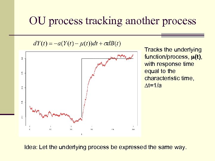 OU process tracking another process Tracks the underlying function/process, (t), with response time equal to the characteristic time, t=1/a Idea: Let the underlying process be expressed the same way.
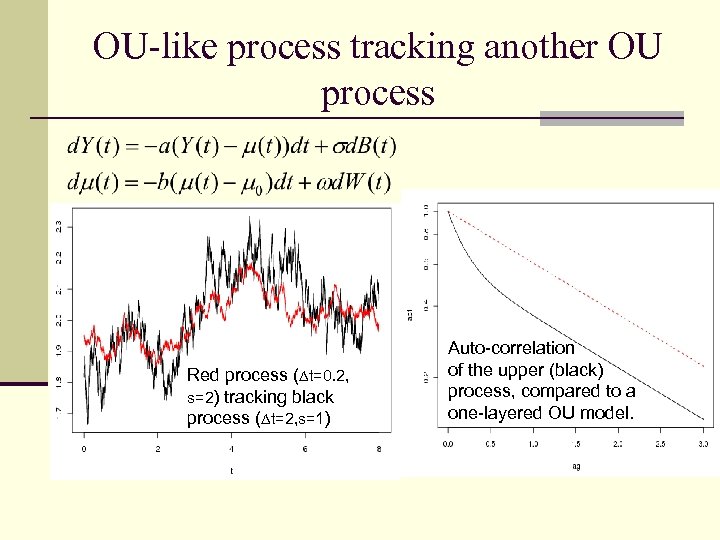 OU-like process tracking another OU process Red process ( t=0. 2, s=2) tracking black process ( t=2, s=1) Auto-correlation of the upper (black) process, compared to a one-layered OU model.
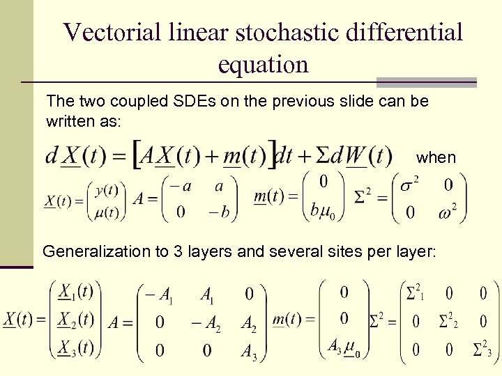 Vectorial linear stochastic differential equation The two coupled SDEs on the previous slide can be written as: when Generalization to 3 layers and several sites per layer:
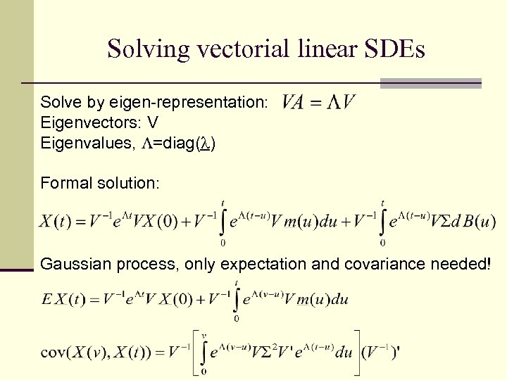 Solving vectorial linear SDEs Solve by eigen-representation: Eigenvectors: V Eigenvalues, =diag( ) Formal solution: Gaussian process, only expectation and covariance needed!
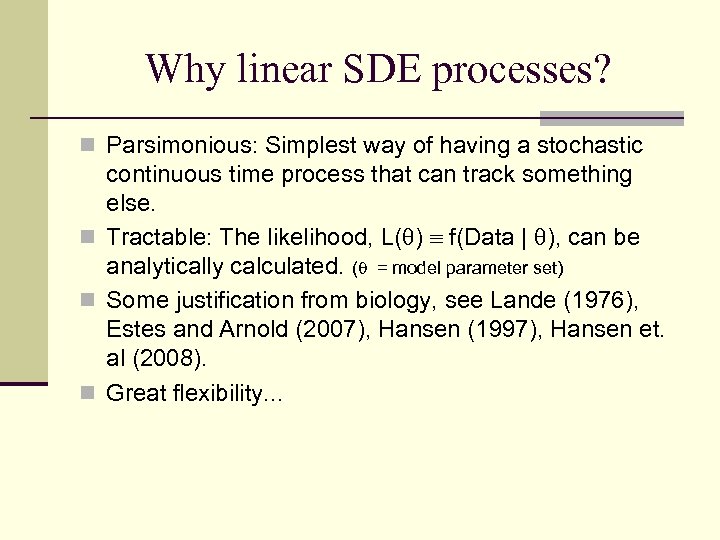 Why linear SDE processes? n Parsimonious: Simplest way of having a stochastic continuous time process that can track something else. n Tractable: The likelihood, L( ) f(Data | ), can be analytically calculated. ( = model parameter set) n Some justification from biology, see Lande (1976), Estes and Arnold (2007), Hansen (1997), Hansen et. al (2008). n Great flexibility. . .
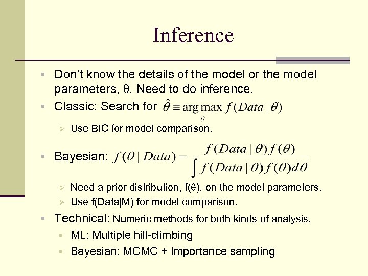 Inference § Don’t know the details of the model or the model parameters, . Need to do inference. § Classic: Search for Ø Use BIC for model comparison. § Bayesian: Ø Ø Need a prior distribution, f( ), on the model parameters. Use f(Data|M) for model comparison. § Technical: Numeric methods for both kinds of analysis. § ML: Multiple hill-climbing § Bayesian: MCMC + Importance sampling
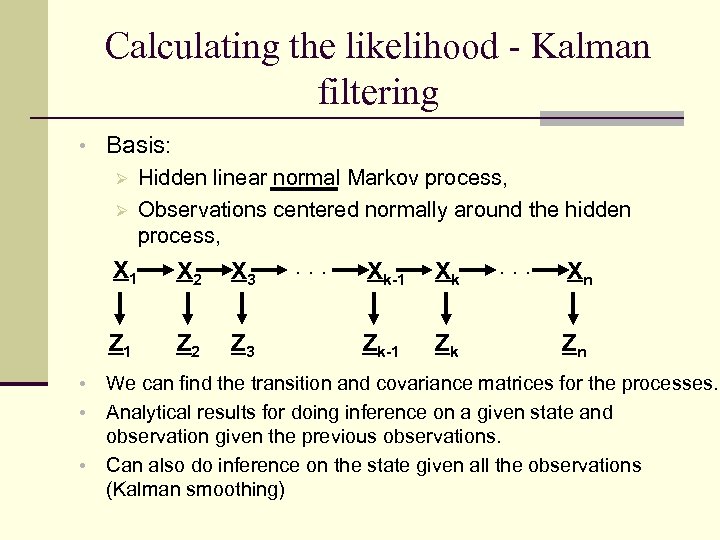 Calculating the likelihood - Kalman filtering • Basis: Ø Hidden linear normal Markov process, Ø Observations centered normally around the hidden process, X 1 • • X 3 Z 1 • X 2 Z 3 . . . Xk-1 Xk Zk-1 Zk . . . Xn Zn We can find the transition and covariance matrices for the processes. Analytical results for doing inference on a given state and observation given the previous observations. Can also do inference on the state given all the observations (Kalman smoothing)
 Do we have enough data for full model selection? • Assume the data has been produced by a given model in this framework. Can we detect it with the given amount of data? Ø How much data is needed in order to reliably detect this by classic and Bayesian means? Ø • Check artificial data against the original model plus 25 likely suspects. • So far: Slight tendency to find the correct number of layers with the Bayesian approach. BIC seems generally too stingy on the number of layers.
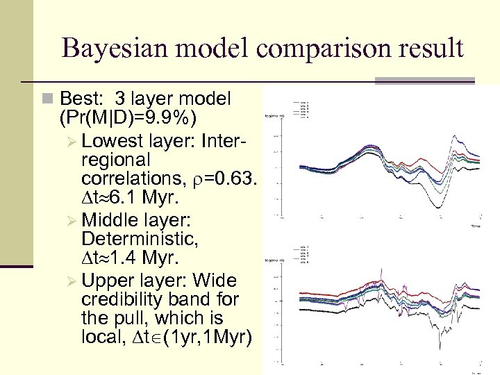 Bayesian model comparison result n Best: 3 layer model (Pr(M|D)=9. 9%) Ø Lowest layer: Interregional correlations, =0. 63. t 6. 1 Myr. Ø Middle layer: Deterministic, t 1. 4 Myr. Ø Upper layer: Wide credibility band for the pull, which is local, t (1 yr, 1 Myr)
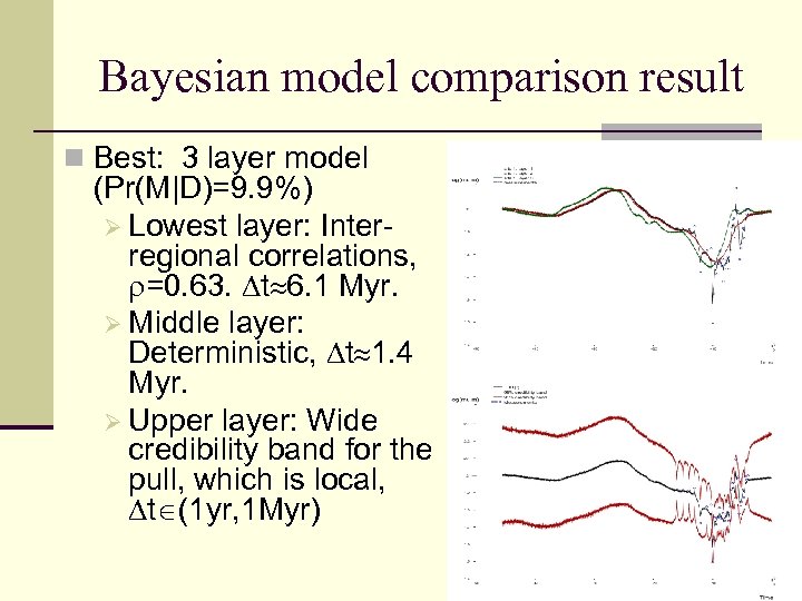 Bayesian model comparison result n Best: 3 layer model (Pr(M|D)=9. 9%) Ø Lowest layer: Interregional correlations, =0. 63. t 6. 1 Myr. Ø Middle layer: Deterministic, t 1. 4 Myr. Ø Upper layer: Wide credibility band for the pull, which is local, t (1 yr, 1 Myr)
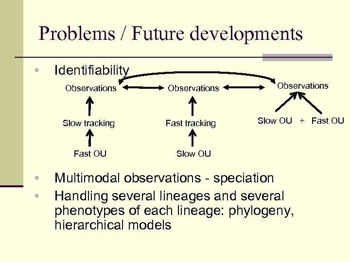 Problems / Future developments § Identifiability Observations Slow tracking Fast OU § § Observations Slow OU + Fast OU Slow OU Multimodal observations - speciation Handling several lineages and several phenotypes of each lineage: phylogeny, hierarchical models
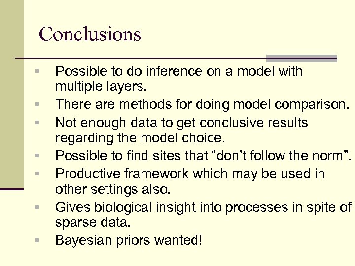 Conclusions § § § § Possible to do inference on a model with multiple layers. There are methods for doing model comparison. Not enough data to get conclusive results regarding the model choice. Possible to find sites that “don’t follow the norm”. Productive framework which may be used in other settings also. Gives biological insight into processes in spite of sparse data. Bayesian priors wanted!
 Links and bibliography n Presentation: http: //folk. uio. no/trondr/stoch_layers 7. ppt http: //folk. uio. no/trondr/stoch_layers 7. pdf n Bibliography: Ø Ø Lande R (1976), Natural Selection and Random Genetic Drift in Phenotypic Evolution, Evolution 30, 314 -334 Hansen TF (1997), Stabilizing Selection and the Comparative Analysis of Adaptation, Evolution, 51 -5, 13411351 Estes S, Arnold SJ (2007), Resolving the Paradox of Stasis: Models with Stabilizing Selection Explain Evolutionary Divergence on All Timescales, The American Naturalist, 1692, 227 -244 Hansen TF, Pienaar J, Orzack SH (2008), A Comparative Method for Studying Adaptation to a Randomly Evolving Environment, Evolution 62 -8, 1965 -1977


