Modelling of dynamic systems Part 2 Solving differential

Скачать презентацию Modelling of dynamic systems Part 2 Solving differential

02e580b75f471768f8220eb86a7acbda.ppt

Количество слайдов: 122

Modelling of dynamic systems: Part 2 Solving differential equations using computers Robert N. Shorten & Douglas Leith The Hamilton Institute NUI Maynooth Robert N. Shorten Hamilton Institute

Contacting me? • How can you contact me? – email: robert. shorten@may. ie – My office is in the Hamilton Institute • When can you ask me questions? – During lectures – Contact hours (any time) • Books – Booklist on the web (www. hamilton. may. ie/~course/) Hamilton Institute

Overview • Lecture 1: Introduction – What are ordinary differential equations? – Why are they important? – Why are they difficult to solve? • Lecture 2: Solving differential equations – Euler’s method • Lecture 3: Solving differential equations – Runge Kutta method • Lecture 4: Systems of differential equations, stiff systems, and some examples Introduction Hamilton Institute

Mathematics! Show no fear - Maths is just another language!! Relax, don’t panic, and think about the equation. Pay attention to detail and pay particular attention to Theorems and to the proofs Hamilton Institute

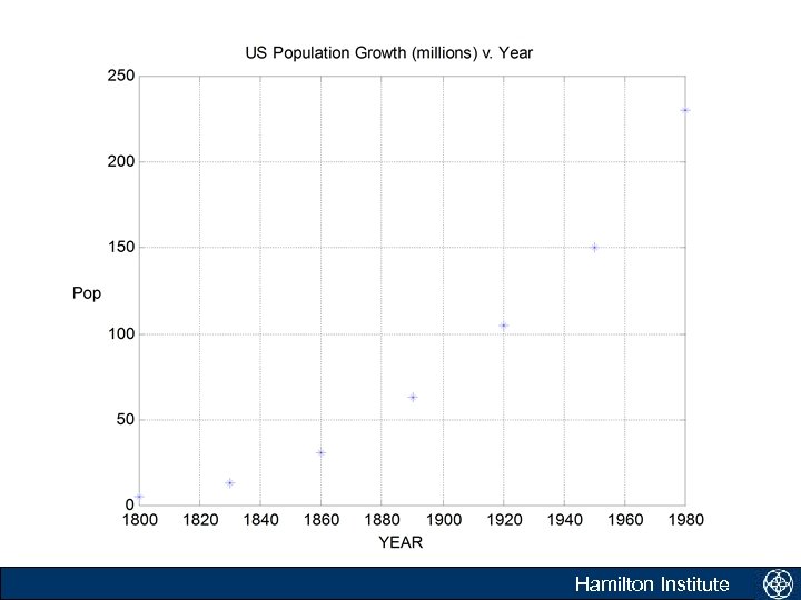
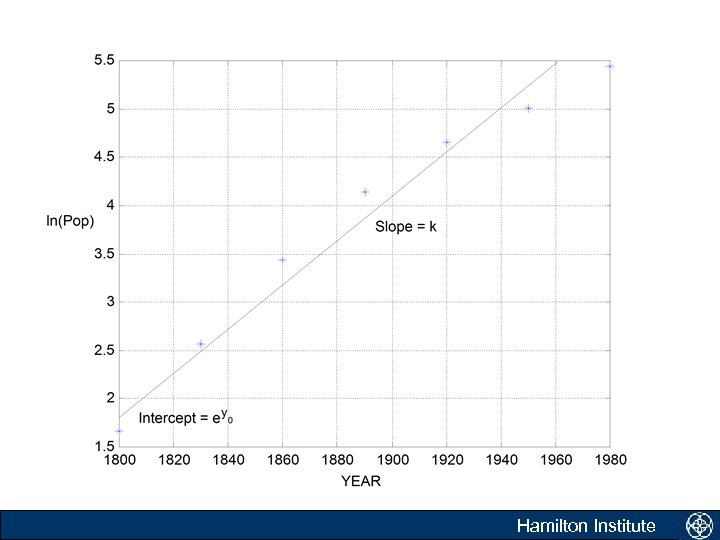
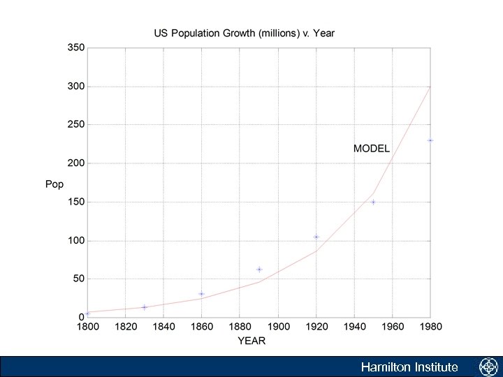
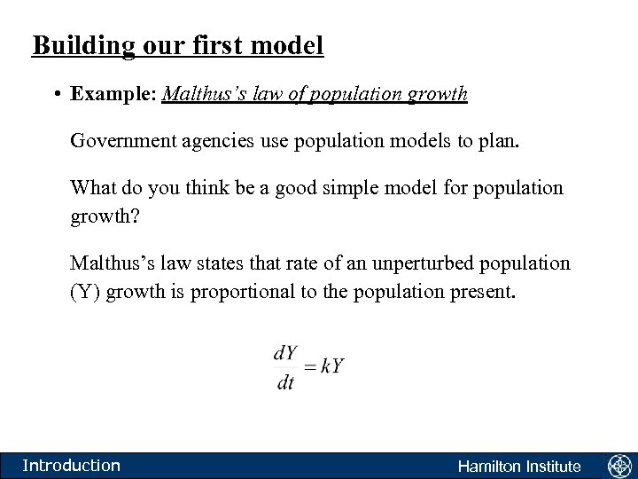Building our first model • Example: Malthus’s law of population growth Government agencies use population models to plan. What do you think be a good simple model for population growth? Malthus’s law states that rate of an unperturbed population (Y) growth is proportional to the population present. Introduction Hamilton Institute

Hamilton Institute

Modelling • Modelling is usually necessary for two reasons: to predict and to control. However to build models we need to do a lot of work. – Postulate the model structure (most physical systems can be classified as belonging to the system classes that you have already seen) – Identify the model parameters (later); – Validate the parameters (later); – Solve the equations to use the model for prediction and analysis (now); Introduction Hamilton Institute

Introduction: How do we predict? • To predict we need to solve our equations: – continuous time systems; discrete time systems; and hybrid systems. – Sometimes, when we are very lucky, we can find an analytic solution to these equations. – More often, an analytic solution cannot be found, and we must use a computer to approximate the solution to the equation. – This is usually not a problem for discrete time systems. However, for continuous systems, modelled using differential equations, life is not so simple. Solving differential equations is the subject of the next four lectures. Introduction Hamilton Institute

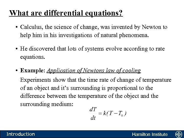What are differential equations? • Calculus, the science of change, was invented by Newton to help him in his investigations of natural phenomena. • He discovered that lots of systems evolve according to rate equations. • Example: Application of Newtons law of cooling Experiments show that the time rate of change of temperature of an object and it’s surrounding is proportional to the difference between the temperature of the object and the surrounding medium: Introduction Hamilton Institute

What are differential equations? • Calculus, the science of change, was invented by Newton to help him in his investigations of natural phenomena. • Many other types of systems can be modelled by writing down an equation for the rate of change of some variable: – – – bandwidth utilisation in TCP networks; acceleration of car; mortgage repayments; population increases; chemical change of some kind; flight of a football; • All of the above behaviour can be captured by very simple differential equations Introduction Hamilton Institute

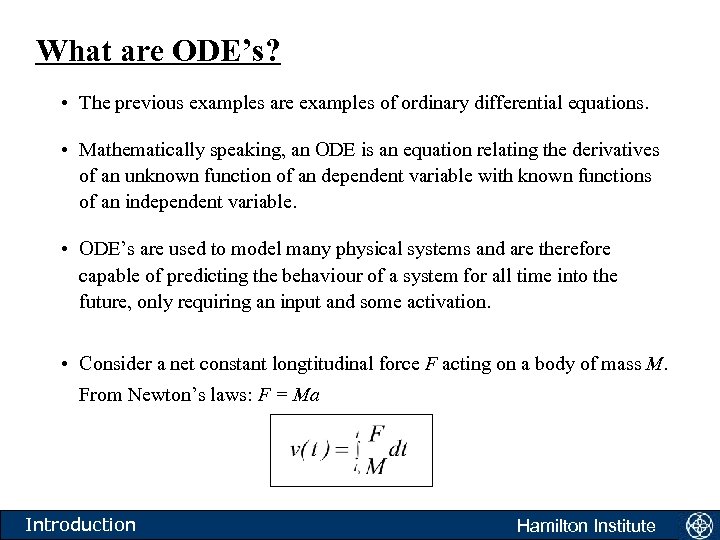What are ODE’s? • The previous examples are examples of ordinary differential equations. • Mathematically speaking, an ODE is an equation relating the derivatives of an unknown function of an dependent variable with known functions of an independent variable. • ODE’s are used to model many physical systems and are therefore capable of predicting the behaviour of a system for all time into the future, only requiring an input and some activation. • Consider a net constant longtitudinal force F acting on a body of mass M. From Newton’s laws: F = Ma Introduction Hamilton Institute

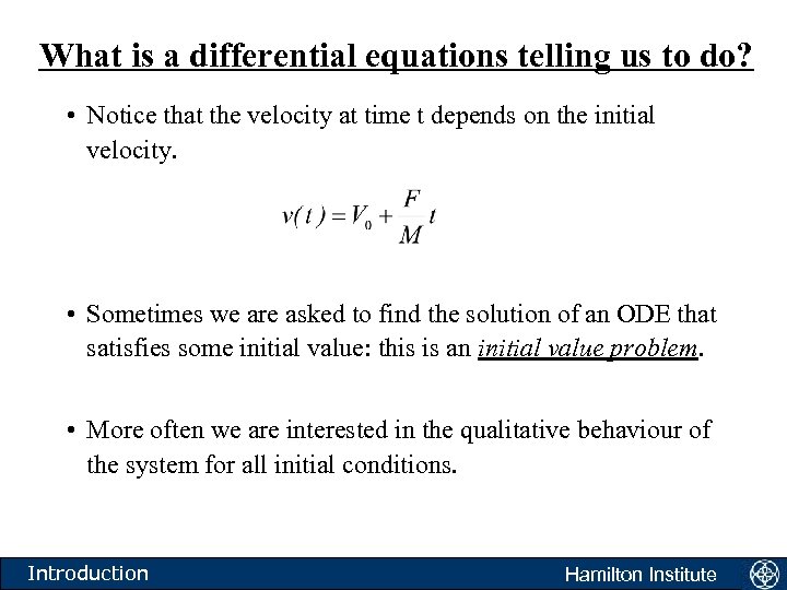What is a differential equations telling us to do? • Notice that the velocity at time t depends on the initial velocity. • Sometimes we are asked to find the solution of an ODE that satisfies some initial value: this is an initial value problem. • More often we are interested in the qualitative behaviour of the system for all initial conditions. Introduction Hamilton Institute

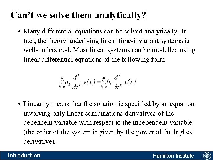Can’t we solve them analytically? • Many differential equations can be solved analytically. In fact, theory underlying linear time-invariant systems is well-understood. Most linear systems can be modelled using linear differential equations of the following form • Linearity means that the solution is specified by an equation involving only linear combinations derivatives of the dependent variable with respect to the independent variable. (the order of the system is given by the power of the highest derivative). Introduction Hamilton Institute

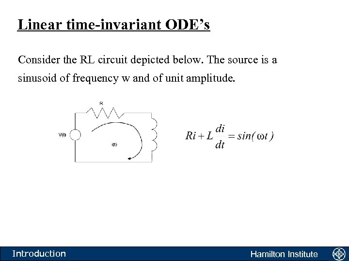Linear time-invariant ODE’s Consider the RL circuit depicted below. The source is a sinusoid of frequency w and of unit amplitude. Introduction Hamilton Institute

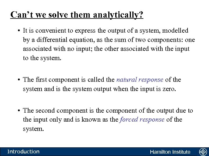Can’t we solve them analytically? • It is convenient to express the output of a system, modelled by a differential equation, as the sum of two components: one associated with no input; the other associated with the input to the system. • The first component is called the natural response of the system and is the system output when the input is zero. • The second component is the component of the output due to the input only and is known as the forced response of the system. Introduction Hamilton Institute

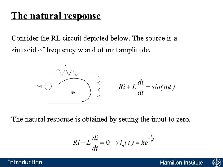The natural response Consider the RL circuit depicted below. The source is a sinusoid of frequency w and of unit amplitude. The natural response is obtained by setting the input to zero. Introduction Hamilton Institute

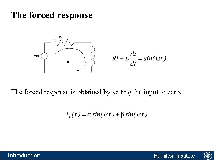The forced response is obtained by setting the input to zero. Introduction Hamilton Institute

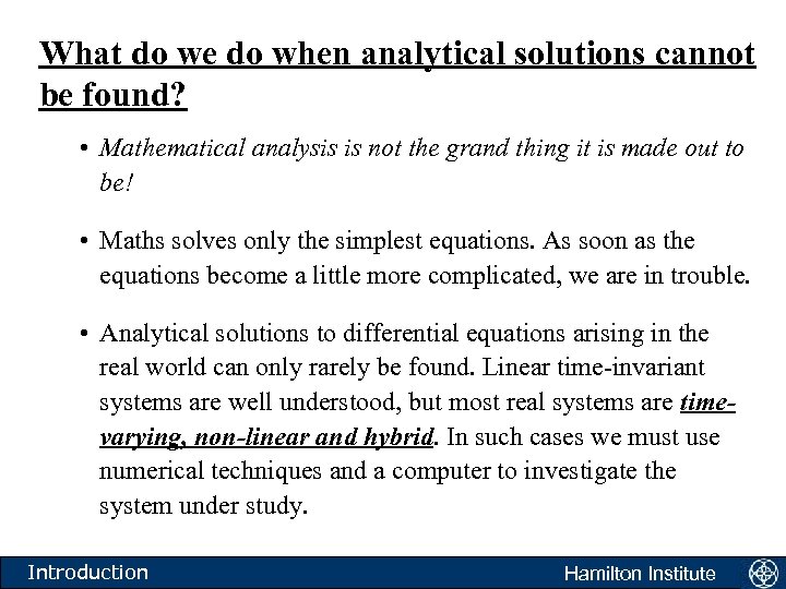
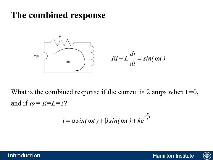The combined response What is the combined response if the current is 2 amps when t =0, and if w = R=L=1? Introduction Hamilton Institute

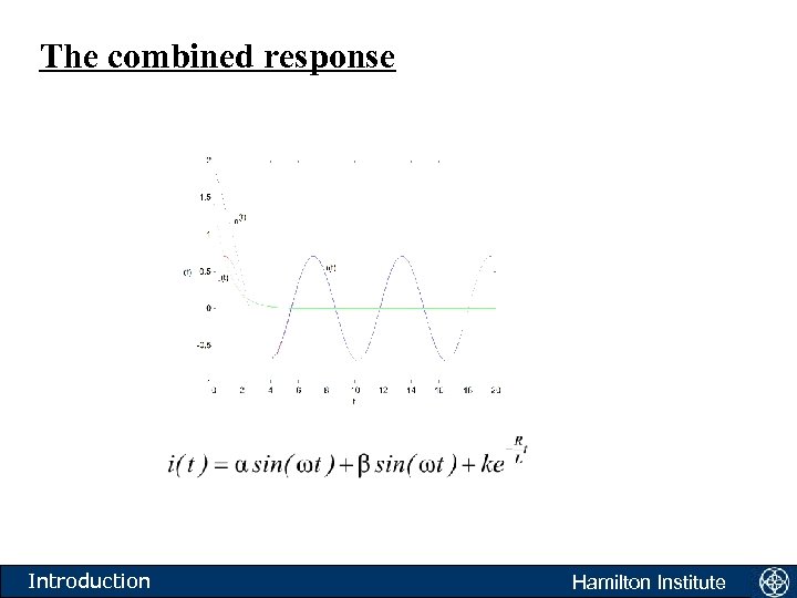The combined response Introduction Hamilton Institute

What do we do when analytical solutions cannot be found? • Mathematical analysis is not the grand thing it is made out to be! • Maths solves only the simplest equations. As soon as the equations become a little more complicated, we are in trouble. • Analytical solutions to differential equations arising in the real world can only rarely be found. Linear time-invariant systems are well understood, but most real systems are timevarying, non-linear and hybrid. In such cases we must use numerical techniques and a computer to investigate the system under study. Introduction Hamilton Institute

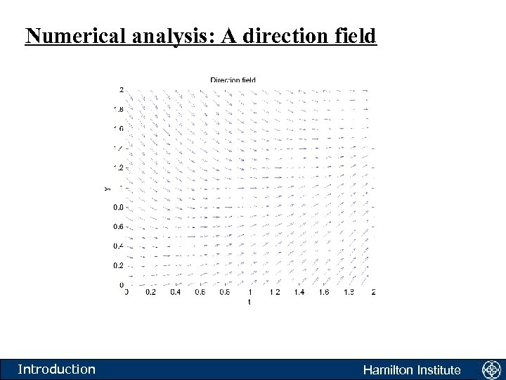
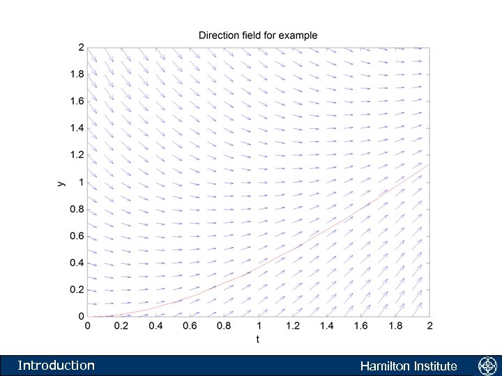
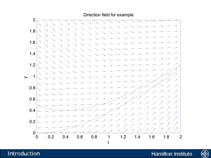
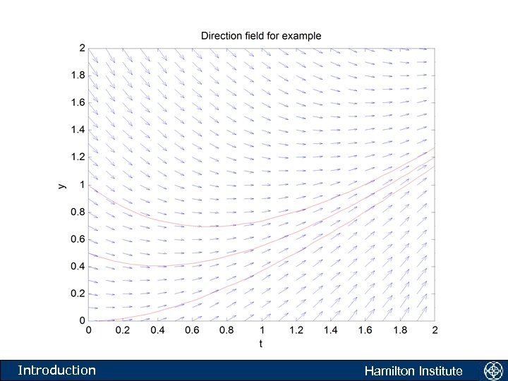
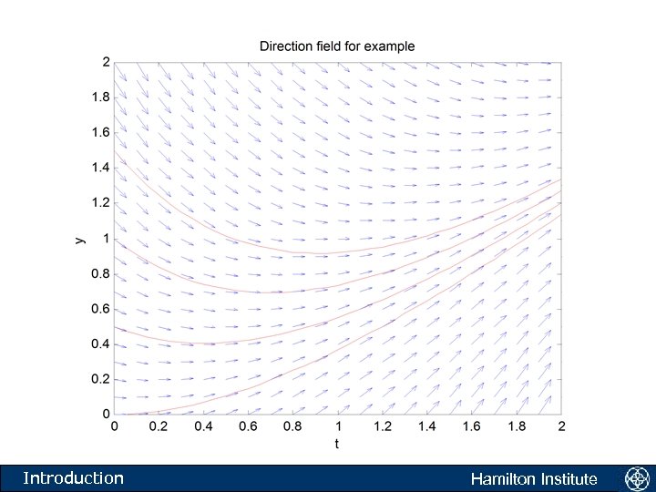
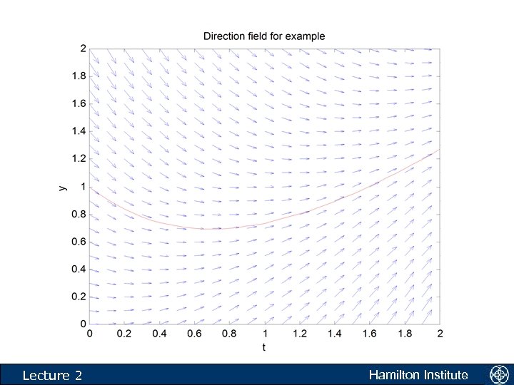
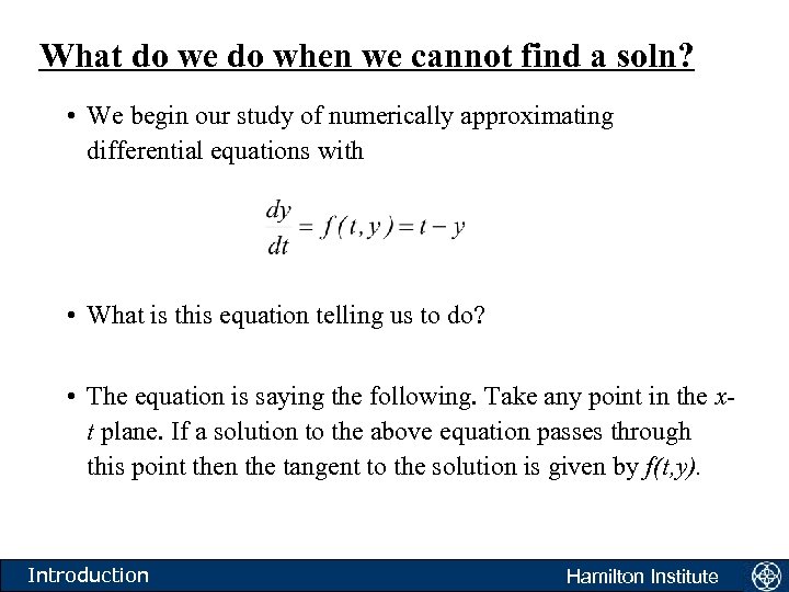What do we do when we cannot find a soln? • We begin our study of numerically approximating differential equations with • What is this equation telling us to do? • The equation is saying the following. Take any point in the xt plane. If a solution to the above equation passes through this point then the tangent to the solution is given by f(t, y). Introduction Hamilton Institute

Numerical analysis: A direction field Introduction Hamilton Institute

Introduction Hamilton Institute

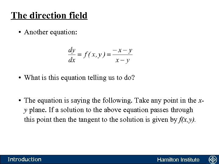The direction field • Another equation: • What is this equation telling us to do? • The equation is saying the following. Take any point in the xy plane. If a solution to the above equation passes through this point then the tangent to the solution is given by f(x, y). Introduction Hamilton Institute

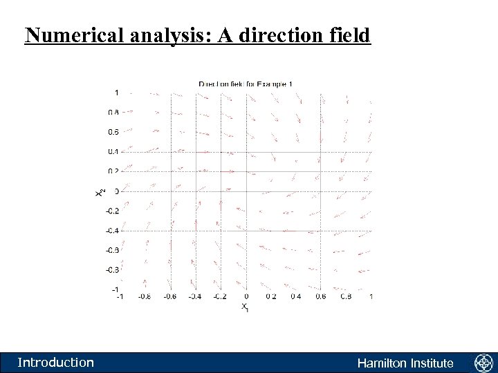Numerical analysis: A direction field Introduction Hamilton Institute

Introduction Hamilton Institute

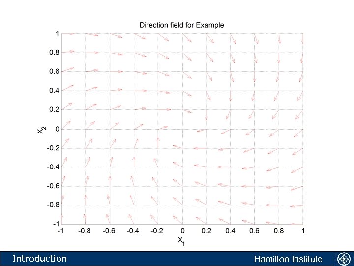
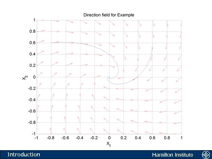
Numerical analysis: Direction fields • We have depicted graphically the directions in which solutions should proceed. • Direction fields generate the flow associated with differential equations. • For such a plot to make sense, the function f(x, y) should satisfy certain properties: it should be defined in some region of the plane; it should be single valued in this region; and solutions to the equation in this region should be differentiable. Introduction Hamilton Institute

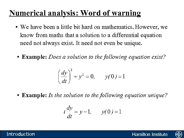Numerical analysis: Word of warning • We have been a little bit hard on mathematics. However, we know from maths that a solution to a differential equation need not always exist. It need not even be unique. • Example: Does a solution to the following equation exist? • Example: Is the solution to the following equation unique? Introduction Hamilton Institute

Numerical analysis: Word of warning • We have been a little bit hard on mathematics. However, we know from maths that a solution to a differential equation need not always exist. It need not even be unique. • Computers don’t care. Always be careful about the output of a program. Generally, the computer will give you an answer; not necessarily the one that you want. • Use mathematical theory to verify simulation. In particular, verify uniqueness and existence conditions are satisfied. Introduction Hamilton Institute

Existence and uniqueness • Existence and uniqueness theorems for ordinary differential equations. You should have done them. What are they? • Roughly speaking: if f(t, y) is continuous in some region of the t-y plane then at least one solution to the differential equation exists; if the partial derivative of f w. r. t y exists and is continuous then the solution is unique. • Revise the concept of Lipschitzness and the existence and uniqueness theorems for ODE’s from part one of the course (if it has been covered). Introduction Hamilton Institute

Modelling of dynamic systems: Part 2 Euler’s method Robert N. Shorten & Douglas Leith The Hamilton Institute NUI Maynooth Robert N. Shorten Hamilton Institute

Overview • We have already spoken about the poor job that mathematics has done in studying differential equations. • Most engineering and scientific problems involve differential equations that cannot be solved analytically. • We can use the direction field to get a solution if the order of the problem is not too high, or if there are not too many independent variables. • What do we do in other cases? Lecture 2 Hamilton Institute

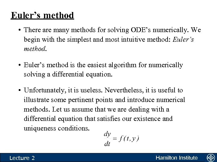Euler’s method • There are many methods for solving ODE’s numerically. We begin with the simplest and most intuitive method: Euler’s method. • Euler’s method is the easiest algorithm for numerically solving a differential equation. • Unfortunately, it is useless. Nevertheless, it is useful to illustrate some pertinent points and introduce numerical methods. Let us assume that we are dealing with a differential equation that satisfies our existence and uniqueness conditions. Lecture 2 Hamilton Institute

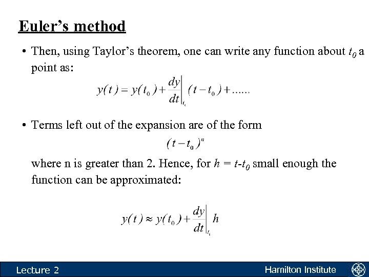Euler’s method • Then, using Taylor’s theorem, one can write any function about t 0 a point as: • Terms left out of the expansion are of the form where n is greater than 2. Hence, for h = t-t 0 small enough the function can be approximated: Lecture 2 Hamilton Institute

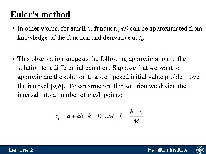Euler’s method • In other words, for small h, function y(t) can be approximated from knowledge of the function and derivative at t 0. • This observation suggests the following approximation to the solution to a differential equation. Suppose that we want to approximate the solution to a well posed initial value problem over the interval [a, b]. To construction this solution we divide the interval into a number of mesh points: Lecture 2 Hamilton Institute

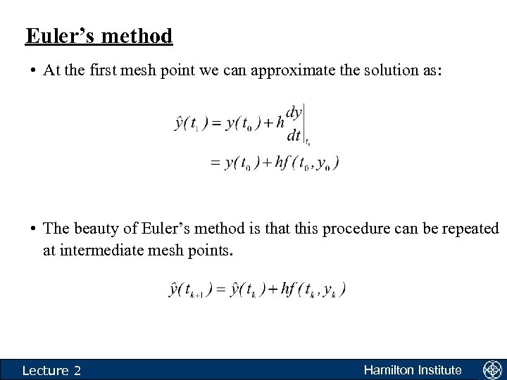Euler’s method • At the first mesh point we can approximate the solution as: • The beauty of Euler’s method is that this procedure can be repeated at intermediate mesh points. Lecture 2 Hamilton Institute

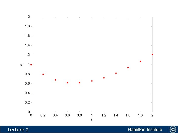
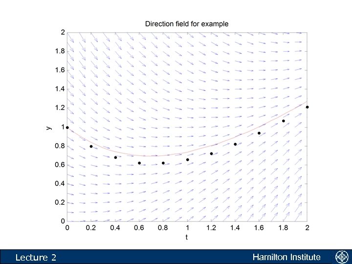
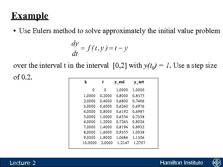Example • Use Eulers method to solve approximately the initial value problem over the interval t in the interval [0, 2] with y(t 0) = 1. Use a step size of 0. 2. k 0 1. 0000 2. 0000 3. 0000 4. 0000 5. 0000 6. 0000 7. 0000 8. 0000 9. 0000 10. 0000 Lecture 2 t 0 0. 2000 0. 4000 0. 6000 0. 8000 1. 0000 1. 2000 1. 4000 1. 6000 1. 8000 2. 0000 y_eul 1. 0000 0. 8000 0. 6800 0. 6240 0. 6192 0. 6554 0. 7243 0. 8194 0. 9355 1. 0684 1. 2147 y_act 1. 0000 0. 8375 0. 7406 0. 6976 0. 6987 0. 7358 0. 8024 0. 8932 1. 0038 1. 1306 1. 2707 Hamilton Institute

k t y_eul 0. 0000 1. 0000 2. 0000 4. 0000 5. 0000 6. 0000 8. 0000 9. 0000 10. 0000 0. 1000 0. 2000 0. 3000 0. 5000 0. 6000 0. 7000 0. 9000 1. 0000 1. 2100 1. 3310 1. 4641 1. 7716 1. 9487 2. 1436 2. 5937 1. 0000 1. 1002 1. 3042 1. 4097 1. 5185 1. 7484 1. 8707 1. 9984 Lecture 2 y_act 3. 0000 7. 0000 0. 4000 0. 8000 1. 1000 1. 6105 2. 3579 1. 2013 1. 6312 2. 1321 Hamilton Institute

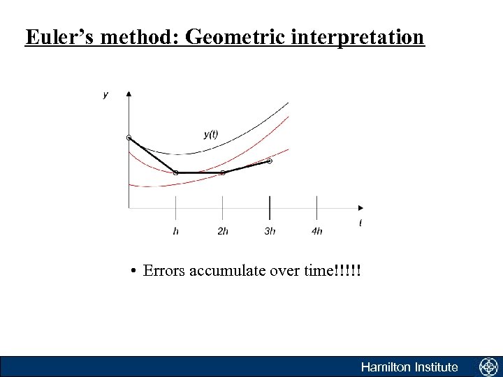Euler’s method: Geometric interpretation • Errors accumulate over time!!!!! Hamilton Institute

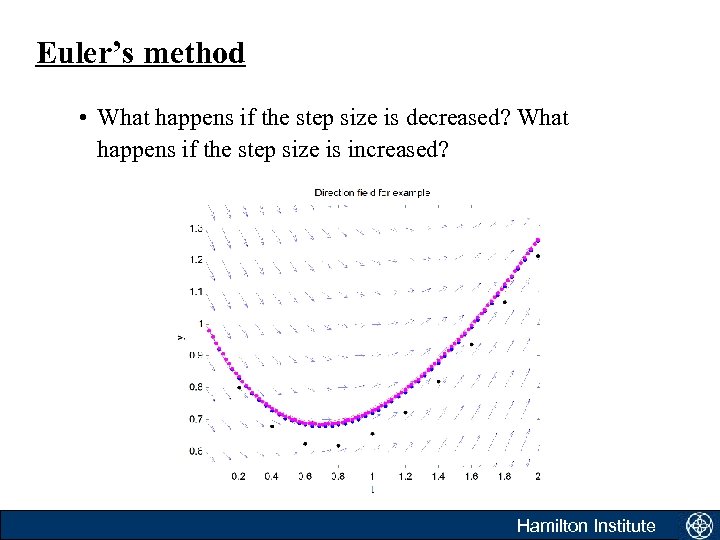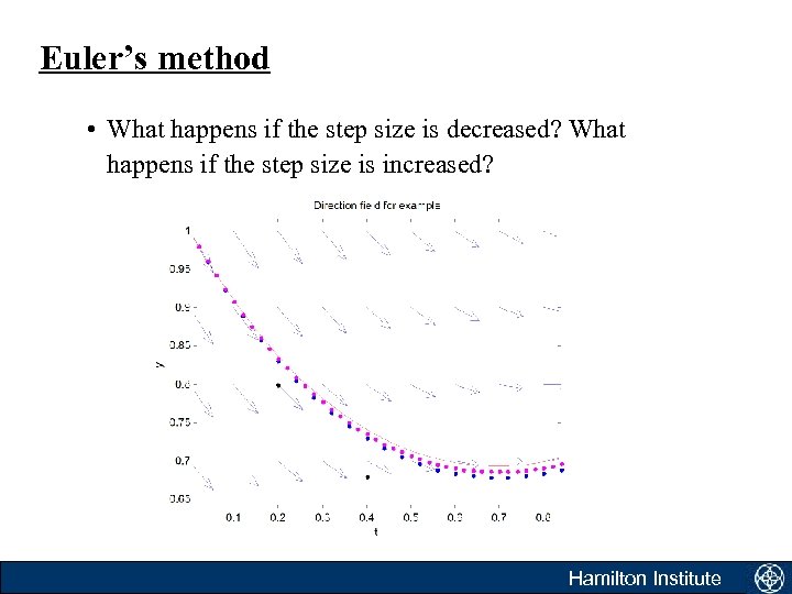Euler’s method • What happens if the step size is decreased? What happens if the step size is increased? Hamilton Institute

Euler’s method: Errors • We have seen that our approximation to the solution to the differential equation is not exact. • Errors are introduced into the procedure as a result of two mechanisms – Round-off – Discretisation errors. • Round-off errors arises from numbers being stored in computers using finite precision. This is usually not a concern as far more error is introduced as a result of truncation. Hamilton Institute

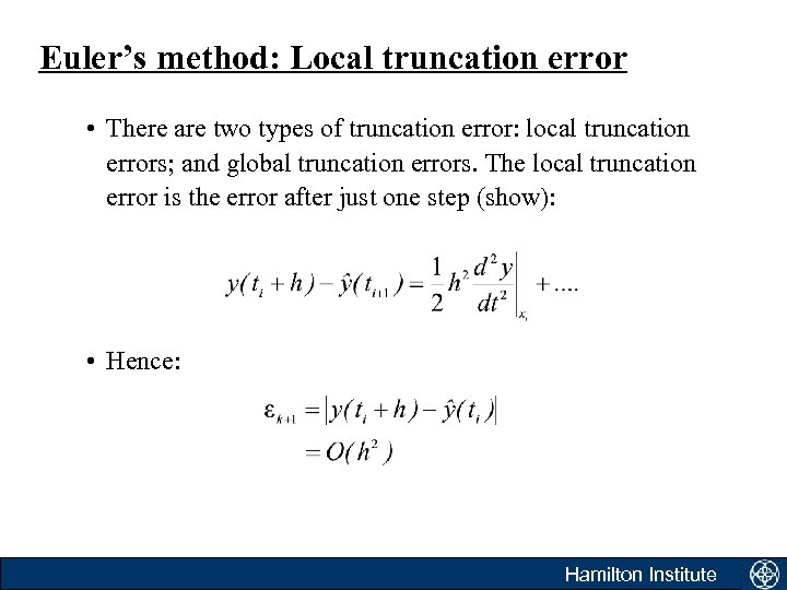Euler’s method: Local truncation error • There are two types of truncation error: local truncation errors; and global truncation errors. The local truncation error is the error after just one step (show): • Hence: Hamilton Institute

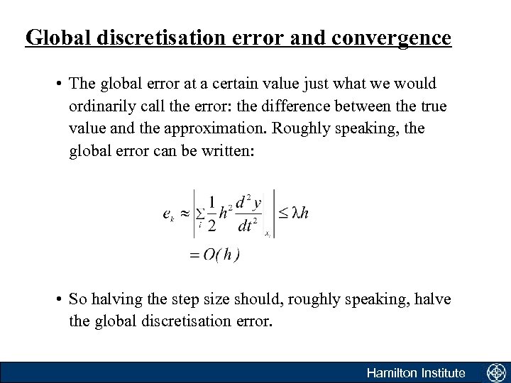Global discretisation error and convergence • The global error at a certain value just what we would ordinarily call the error: the difference between the true value and the approximation. Roughly speaking, the global error can be written: • So halving the step size should, roughly speaking, halve the global discretisation error. Hamilton Institute

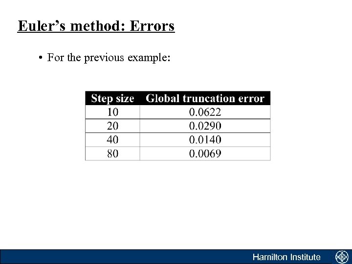Euler’s method: Errors • For the previous example: Hamilton Institute

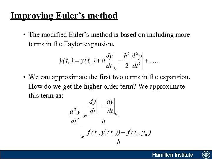Improving Euler’s method • The modified Euler’s method is based on including more terms in the Taylor expansion. • We can approximate the first two terms in the expansion. How do we get the higher order term? We approximate this term as: Hamilton Institute

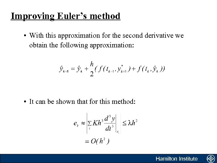Improving Euler’s method • With this approximation for the second derivative we obtain the following approximation: • It can be shown that for this method: Hamilton Institute

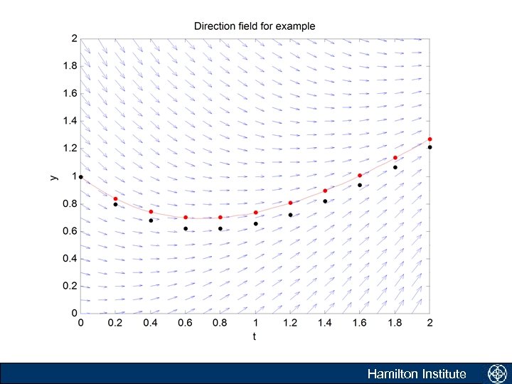Improving Euler’s method Hamilton Institute

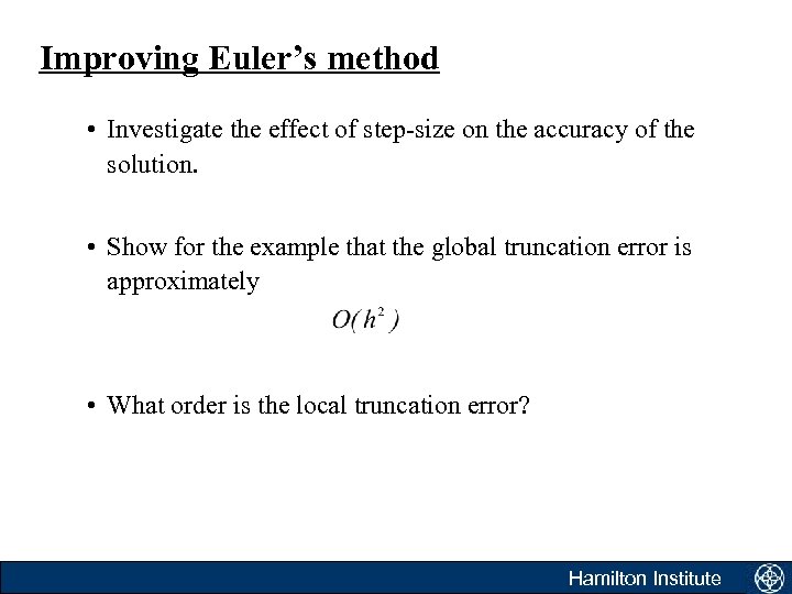Improving Euler’s method • Investigate the effect of step-size on the accuracy of the solution. • Show for the example that the global truncation error is approximately • What order is the local truncation error? Hamilton Institute

Modelling of dynamic systems: Part 2 Runge-Kutta method’s Robert N. Shorten & Douglas Leith The Hamilton Institute NUI Maynooth Robert N. Shorten Hamilton Institute

Overview • In the last lecture we have looked at the Euler method. Euler’s method is usually not good enough. The main reason is that the error is global O(h). • An improvement in the Euler method was obtained through the modified Euler method. • Let’s take a another approach to finding the numerical solution of the differential equation. Lecture 2 Hamilton Institute

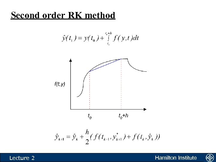Second order RK method Lecture 2 Hamilton Institute

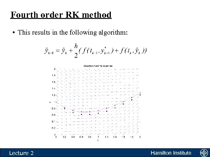Fourth order RK method • This results in the following algorithm: Lecture 2 Hamilton Institute

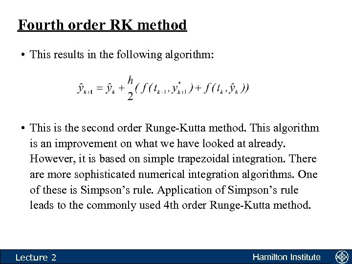Fourth order RK method • This results in the following algorithm: • This is the second order Runge-Kutta method. This algorithm is an improvement on what we have looked at already. However, it is based on simple trapezoidal integration. There are more sophisticated numerical integration algorithms. One of these is Simpson’s rule. Application of Simpson’s rule leads to the commonly used 4 th order Runge-Kutta method. Lecture 2 Hamilton Institute

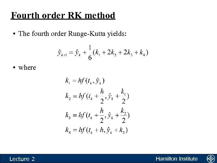Fourth order RK method • The fourth order Runge-Kutta yields: • where Lecture 2 Hamilton Institute

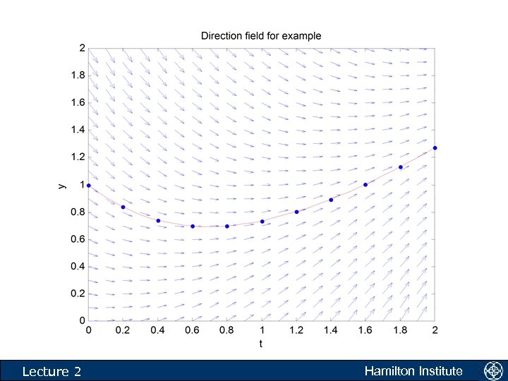
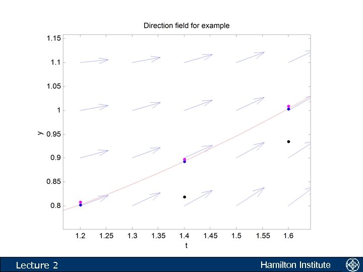
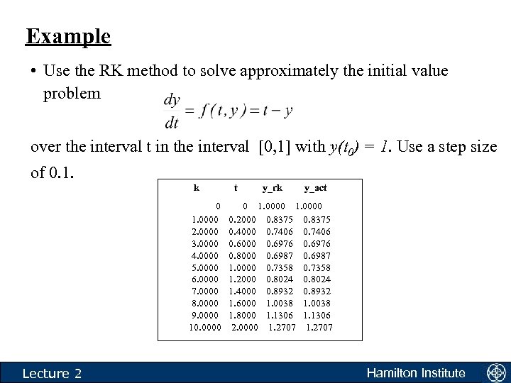Example • Use the RK method to solve approximately the initial value problem over the interval t in the interval [0, 1] with y(t 0) = 1. Use a step size of 0. 1. k 0 1. 0000 2. 0000 3. 0000 4. 0000 5. 0000 6. 0000 7. 0000 8. 0000 9. 0000 10. 0000 Lecture 2 t y_rk y_act 0 1. 0000 0. 2000 0. 8375 0. 4000 0. 7406 0. 6000 0. 6976 0. 8000 0. 6987 1. 0000 0. 7358 1. 2000 0. 8024 1. 4000 0. 8932 1. 6000 1. 0038 1. 8000 1. 1306 2. 0000 1. 2707 Hamilton Institute

k 0 1. 0000 2. 0000 3. 0000 4. 0000 5. 0000 6. 0000 7. 0000 8. 0000 9. 0000 10. 0000 Lecture 2 t 0 0. 2000 0. 4000 0. 6000 0. 8000 1. 0000 1. 2000 1. 4000 1. 6000 1. 8000 2. 0000 y_eul 1. 0000 0. 8000 0. 6800 0. 6240 0. 6192 0. 6554 0. 7243 0. 8194 0. 9355 1. 0684 1. 2147 y_act 1. 0000 0. 8375 0. 7406 0. 6976 0. 6987 0. 7358 0. 8024 0. 8932 1. 0038 1. 1306 1. 2707 Hamilton Institute

Lecture 2 Hamilton Institute

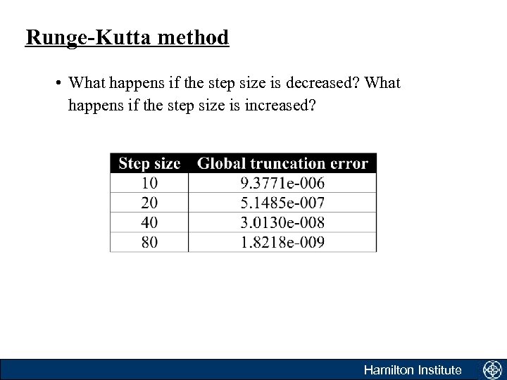Runge-Kutta method • What happens if the step size is decreased? What happens if the step size is increased? Hamilton Institute

Fourth order Runge-Kutta method • The fourth order Runge-Kutta is very popular for a variety of reasons. 1) It is simple to program. 2) It is very accurate. The global truncation error is O(h 4). The local truncation error is O(h 5). 3) It is very efficient. Hamilton Institute

A few words on stability • All of the methods that we have considered were of the form: • This is a first order difference equation and will be unstable (when)? • If we keep the step size small enough then we can usually ensure stability. Hamilton Institute

Efficiency of the RK schemes • We have said that the 4 th order RK method is more efficient than other techniques that we have considered. • How do me measure efficiency? There are two components to consider. – Computational effort; – Truncation errors. • We get a rough measure of computational effort by counting how many times the function f(t, y) is evaluated as we make a prediction to a desired accuracy. Hamilton Institute

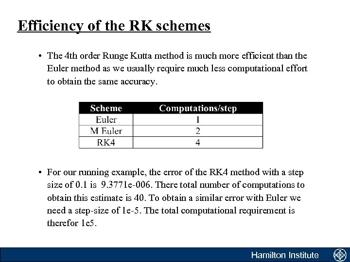Efficiency of the RK schemes • The 4 th order Runge Kutta method is much more efficient than the Euler method as we usually require much less computational effort to obtain the same accuracy. • For our running example, the error of the RK 4 method with a step size of 0. 1 is 9. 3771 e-006. There total number of computations to obtain this estimate is 40. To obtain a similar error with Euler we need a step-size of 1 e-5. The total computational requirement is therefor 1 e 5. Hamilton Institute

Runge-Kutta-Fehlberg • The big problem when using any method is to estimate the accuracy of the approximation (the global truncation error). • Normally we do not have access to the solution so the problem is not straight forward. • One approach to estimate the accuracy of the solution was proposed by Fehlberg. Hamilton Institute

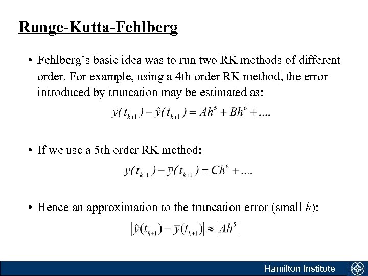Runge-Kutta-Fehlberg • Fehlberg’s basic idea was to run two RK methods of different order. For example, using a 4 th order RK method, the error introduced by truncation may be estimated as: • If we use a 5 th order RK method: • Hence an approximation to the truncation error (small h): Hamilton Institute

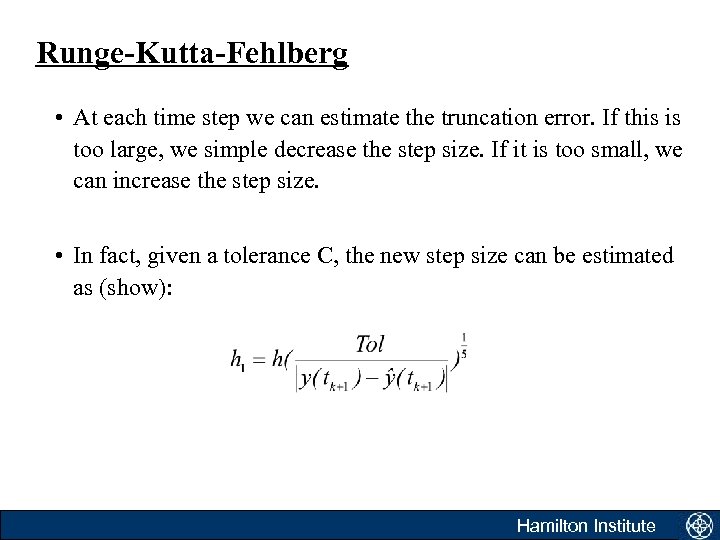Runge-Kutta-Fehlberg • At each time step we can estimate the truncation error. If this is too large, we simple decrease the step size. If it is too small, we can increase the step size. • In fact, given a tolerance C, the new step size can be estimated as (show): Hamilton Institute

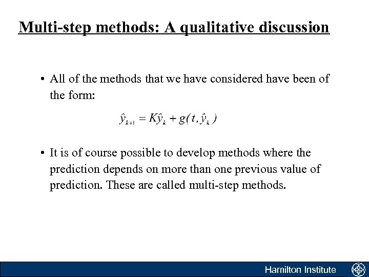Multi-step methods: A qualitative discussion • All of the methods that we have considered have been of the form: • It is of course possible to develop methods where the prediction depends on more than one previous value of prediction. These are called multi-step methods. Hamilton Institute

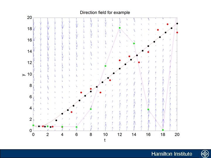
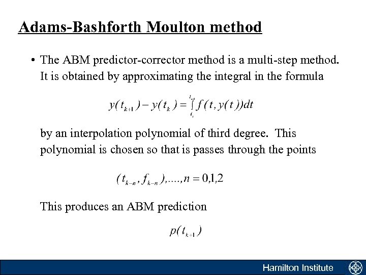Adams-Bashforth Moulton method • The ABM predictor-corrector method is a multi-step method. It is obtained by approximating the integral in the formula by an interpolation polynomial of third degree. This polynomial is chosen so that is passes through the points This produces an ABM prediction Hamilton Institute

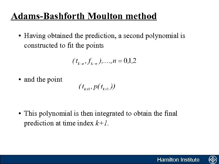Adams-Bashforth Moulton method • Having obtained the prediction, a second polynomial is constructed to fit the points • and the point • This polynomial is then integrated to obtain the final prediction at time index k+1. Hamilton Institute

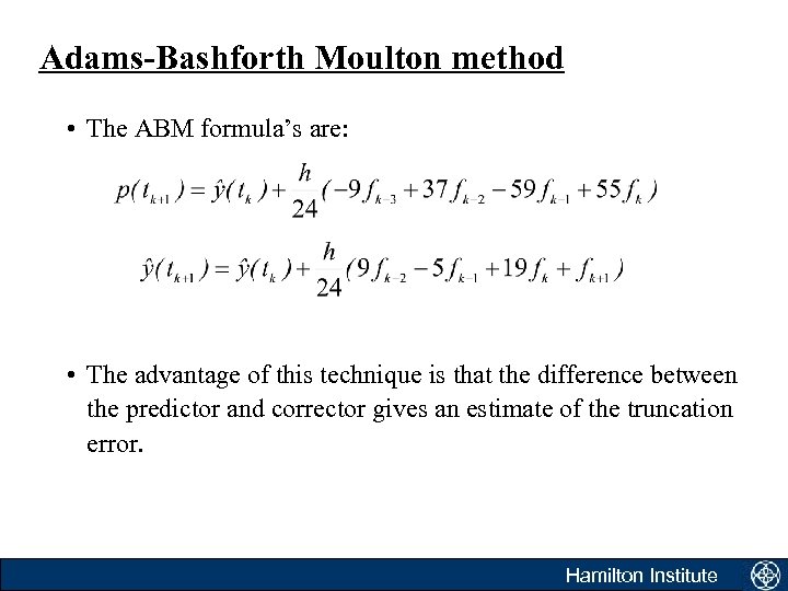Adams-Bashforth Moulton method • The ABM formula’s are: • The advantage of this technique is that the difference between the predictor and corrector gives an estimate of the truncation error. Hamilton Institute

Adams-Bashforth-Moulton method • Disadvantages of the technique include (1) The first 4 predictions must be obtained using some other method. (2)The technique results in a high order difference equation. Care must be taken to ensure that this equation remains stable (zeros inside the unit circle). Hamilton Institute

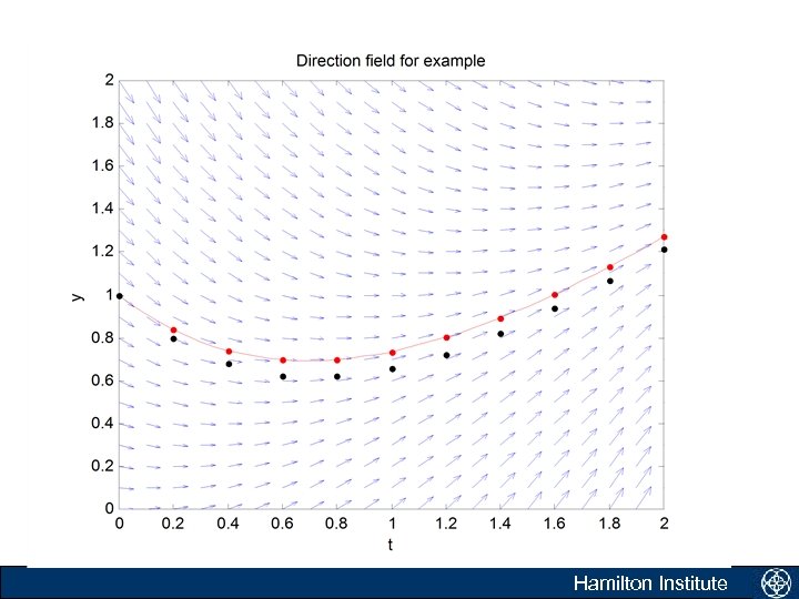Adams-Bashforth-Moulton method Hamilton Institute

Examples • Eulers method • Modified Euler method • 4 th order Runge-Kutta method Hamilton Institute

Modelling of dynamic systems: Part 2 Systems of differential equations Robert N. Shorten & Douglas Leith The Hamilton Institute NUI Maynooth Robert N. Shorten Hamilton Institute

Is the world first order? • Up to now we have considered approximating the solution to first order ordinary differential equations using numerical methods. Our methods work for nonlinear systems and for time-varying systems. • What about second order systems? • What about higher order systems in general? • What about systems of ODE’s? Hamilton Institute

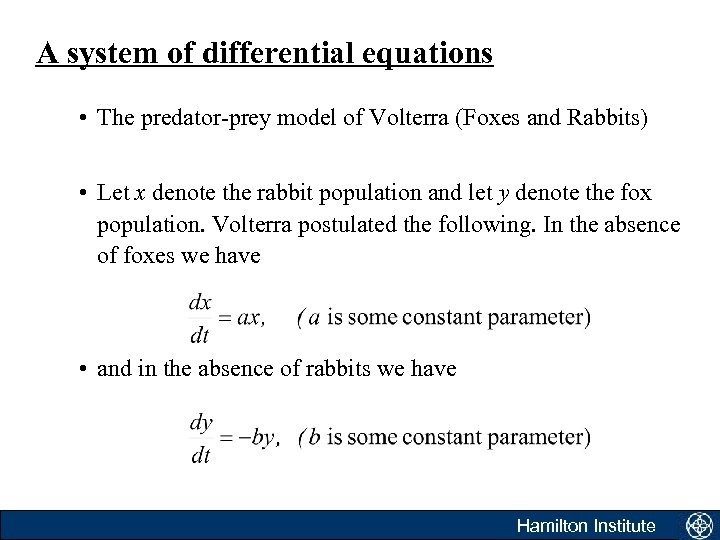A system of differential equations • The predator-prey model of Volterra (Foxes and Rabbits) • Let x denote the rabbit population and let y denote the fox population. Volterra postulated the following. In the absence of foxes we have • and in the absence of rabbits we have Hamilton Institute

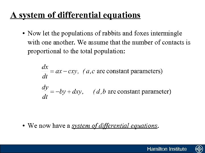A system of differential equations • Now let the populations of rabbits and foxes intermingle with one another. We assume that the number of contacts is proportional to the total population: • We now have a system of differential equations. Hamilton Institute

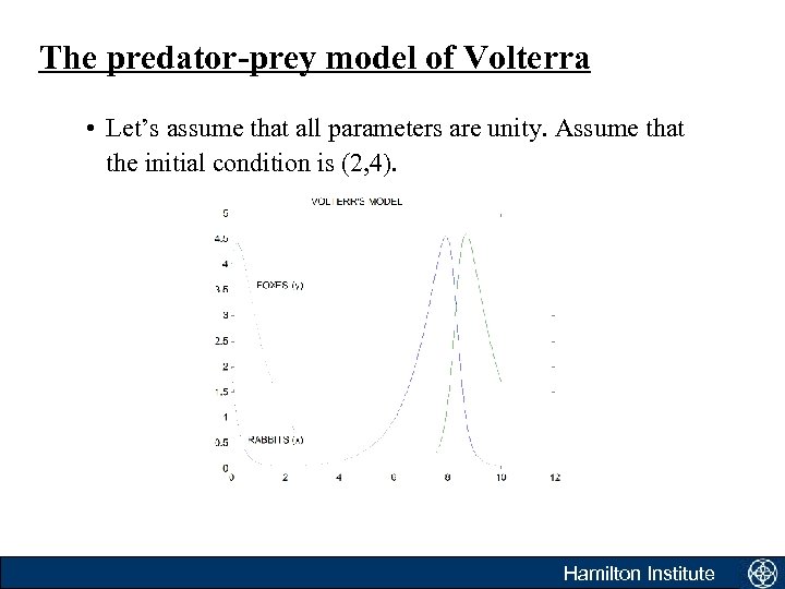The predator-prey model of Volterra • Let’s assume that all parameters are unity. Assume that the initial condition is (2, 4). Hamilton Institute

Higher order equations Hamilton Institute

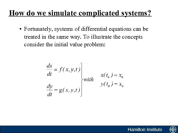How do we simulate complicated systems? • Fortunately, systems of differential equations can be treated in the same way. To illustrate the concepts consider the initial value problem: Hamilton Institute

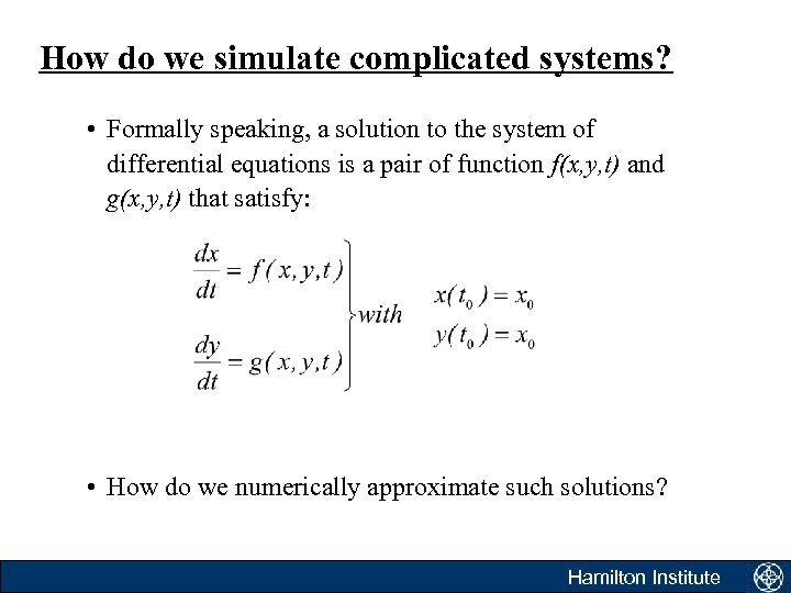How do we simulate complicated systems? • Formally speaking, a solution to the system of differential equations is a pair of function f(x, y, t) and g(x, y, t) that satisfy: • How do we numerically approximate such solutions? Hamilton Institute

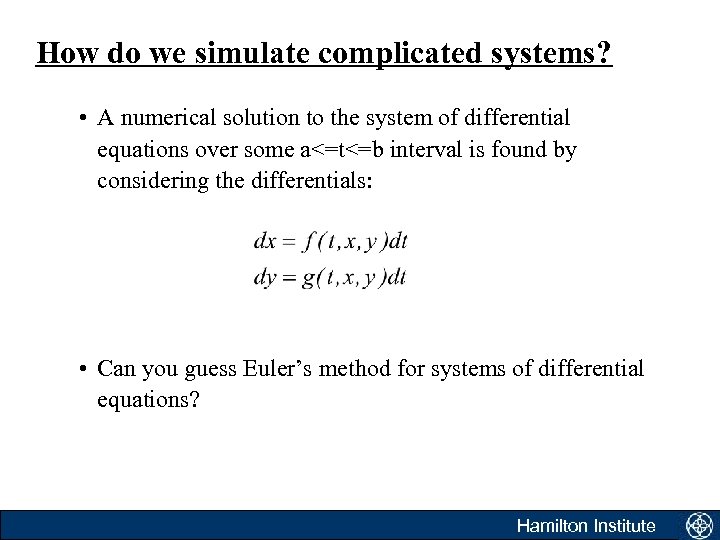How do we simulate complicated systems? • A numerical solution to the system of differential equations over some a<=t<=b interval is found by considering the differentials: • Can you guess Euler’s method for systems of differential equations? Hamilton Institute

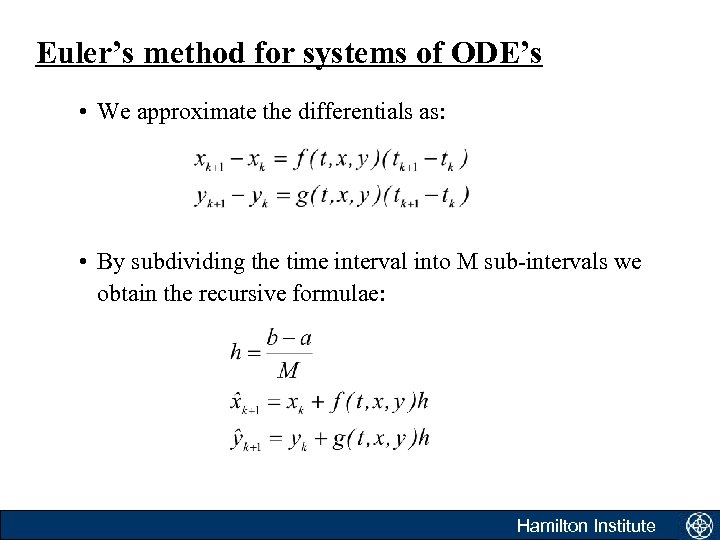Euler’s method for systems of ODE’s • We approximate the differentials as: • By subdividing the time interval into M sub-intervals we obtain the recursive formulae: Hamilton Institute

The predator-prey model of Volterra • Let’s assume that all parameters are unity. Assume that the initial condition is (2, 4). Hamilton Institute

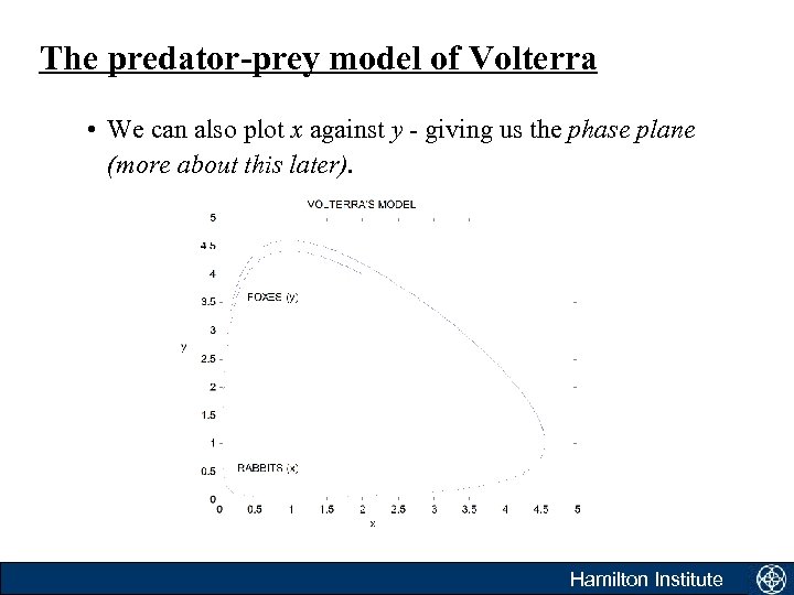The predator-prey model of Volterra • We can also plot x against y - giving us the phase plane (more about this later). Hamilton Institute

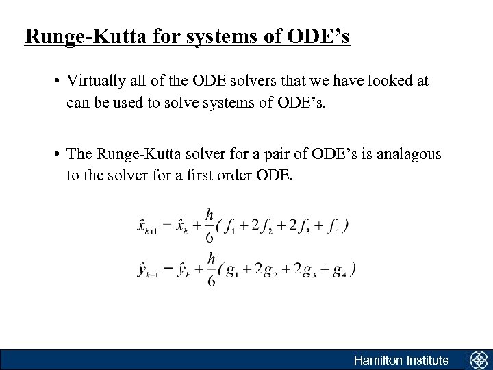Runge-Kutta for systems of ODE’s • Virtually all of the ODE solvers that we have looked at can be used to solve systems of ODE’s. • The Runge-Kutta solver for a pair of ODE’s is analagous to the solver for a first order ODE. Hamilton Institute

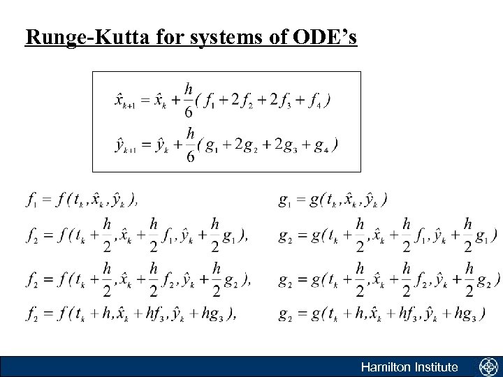Runge-Kutta for systems of ODE’s Hamilton Institute

Systems of differential equations • Virtually all ODE solvers can be extended to solve systems of differential equations. • We have considered (briefly) systems of two equations. Exactly the same methodology applies to systems of more than two equations. • When comparing ODE solvers, the issues that are relevant for first order equations are also relevant for systems of equations. Can you think of any issues that are special to systems of equations? Hamilton Institute

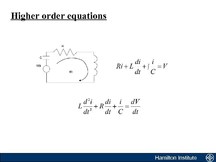
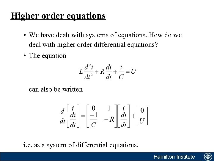Higher order equations • We have dealt with systems of equations. How do we deal with higher order differential equations? • The equation can also be written i. e. as a system of differential equations. Hamilton Institute

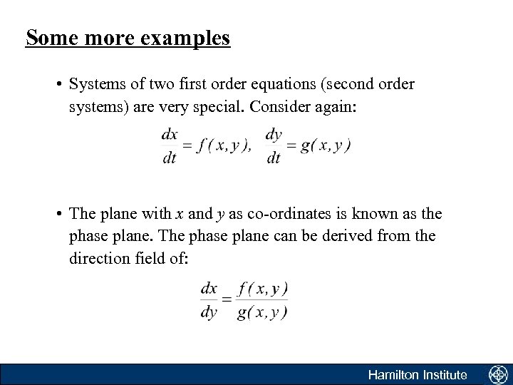Some more examples • Systems of two first order equations (second order systems) are very special. Consider again: • The plane with x and y as co-ordinates is known as the phase plane. The phase plane can be derived from the direction field of: Hamilton Institute

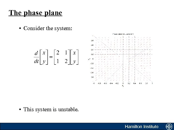The phase plane • Consider the system: • This system is unstable. Hamilton Institute

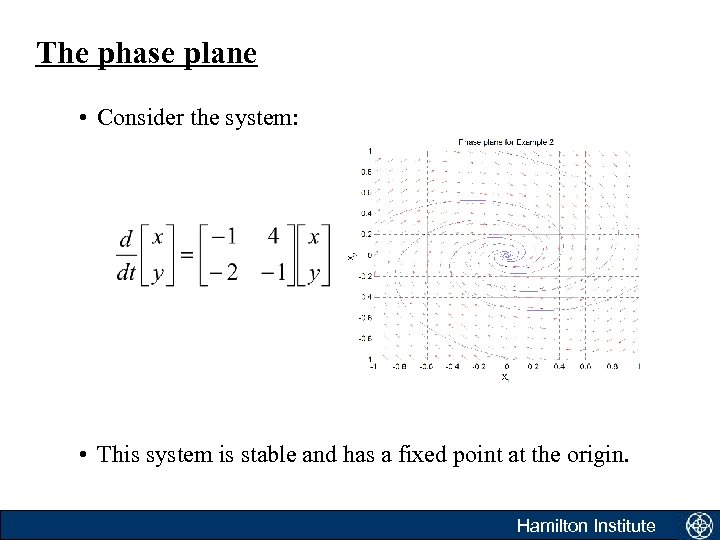The phase plane • Consider the system: • This system is stable and has a fixed point at the origin. Hamilton Institute

A word of warning: Stiff systems • We have already encountered stability problems when looking at first order ODE’s. • Roughly speaking, stability is maintained by choosing a very small step size. • However, very small step-sizes lead to large computational burdens. Hamilton Institute

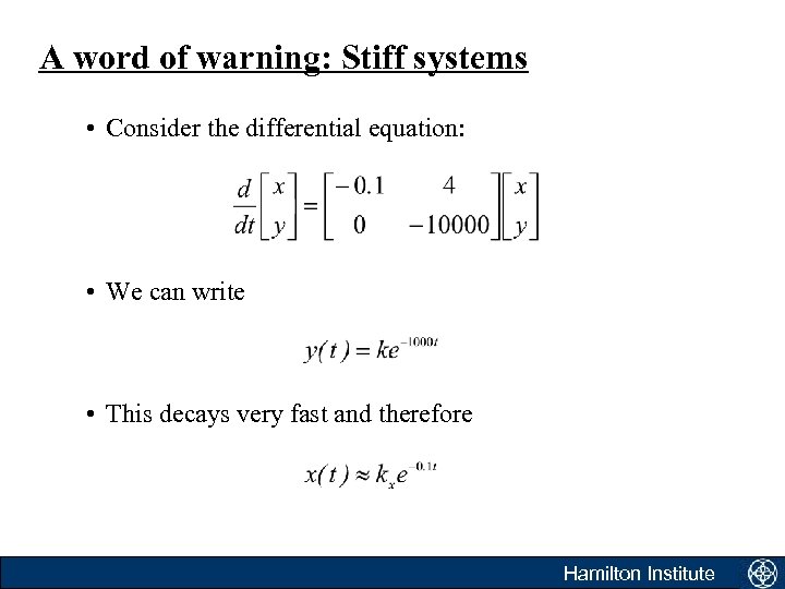A word of warning: Stiff systems • Consider the differential equation: • We can write • This decays very fast and therefore Hamilton Institute

A word of warning: Stiff systems • So, given that y(t) is not that important, we should choose the step-size to approximate: • WRONG!!!!! The stability of the numerical integration is determined by the largest eigenvalue of the system. Always choose a step-size to guarantee stability. • This is an example of a stiff system; a number of variables evolving at different time scales. There are special solvers for such systems. Hamilton Institute

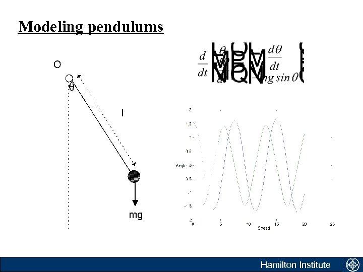
Examples • To finish this part of the course we give two examples where numerical solutions to systems of ODE’s are required. 1) [Physics] Modelling a pendulum A non-linear continuous time system 2) [Computer Science] Network congestion control A system with continuous/discrete state A hybrid systems model (Hespanha) Hamilton Institute

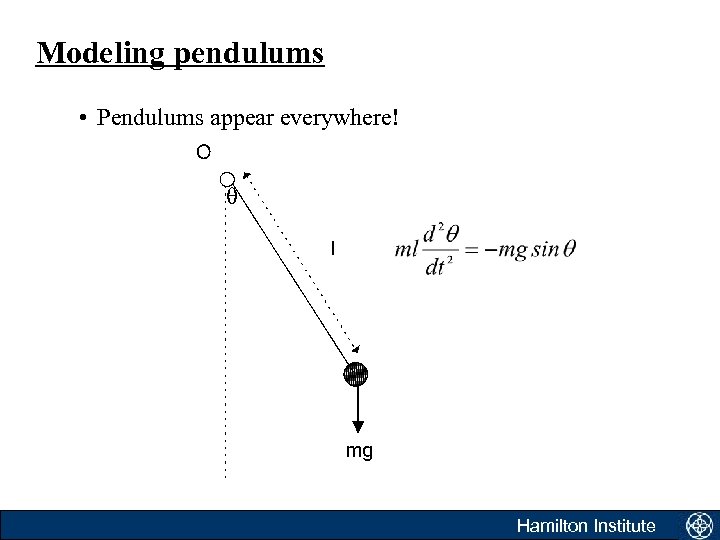Modeling pendulums • Pendulums appear everywhere! Hamilton Institute

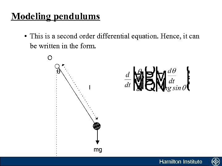Modeling pendulums • This is a second order differential equation. Hence, it can be written in the form. Hamilton Institute

Modeling pendulums Hamilton Institute

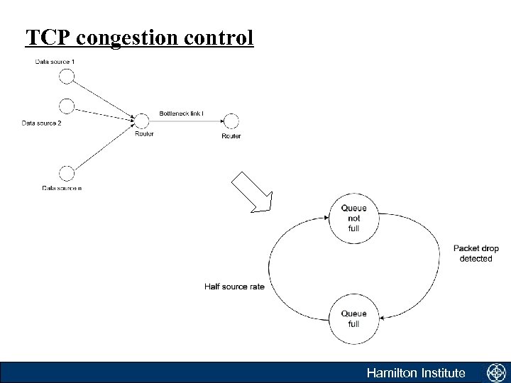
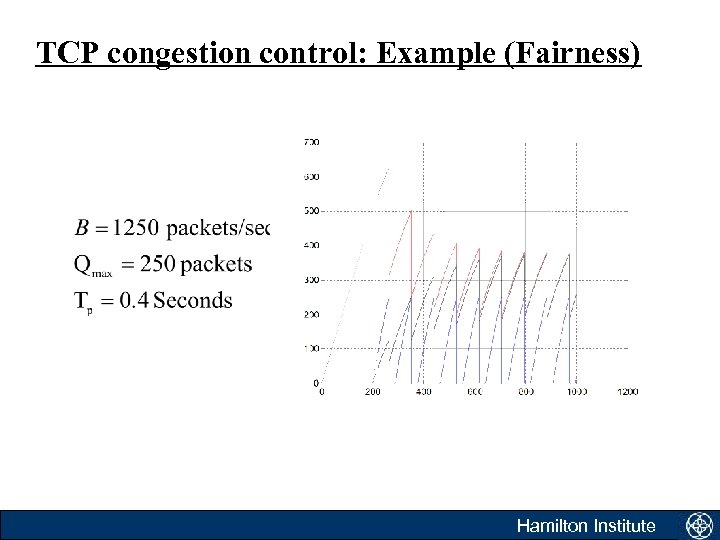
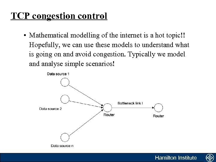TCP congestion control • Mathematical modelling of the internet is a hot topic!! Hopefully, we can use these models to understand what is going on and avoid congestion. Typically we model and analyse simple scenarios! Hamilton Institute

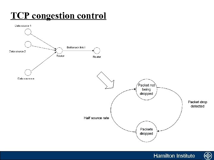
TCP congestion control • Roughly speaking, TCP operates as follows: – Data packets reaching a destination are acknowledged by sending an appropriate message to the sender. – Upon receipt of the acknowledgement, data sources increase their send rate, thereby probing the network for available bandwidth, until congestion is encountered. – Network congestion is deduced through the loss of data packets (receipt of duplicate ACK’s or non receipt of ACK’s), and results in sources reducing their send rate drastically (by half). Hamilton Institute

TCP congestion control • Congestion control is necessary for a number of reasons, so that: – catastrophic collapse of the network is avoided under heavy loads; – each data source receives a fair share of the available bandwidth; – the available bandwidth B is utilised in an optimal fashion. – interactions of the network sources should not cause destabilising network side effects such as oscillations or instability Hamilton Institute

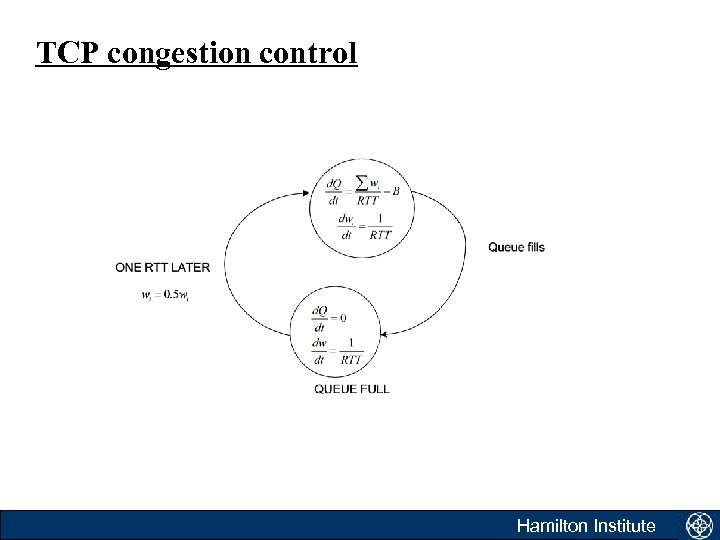
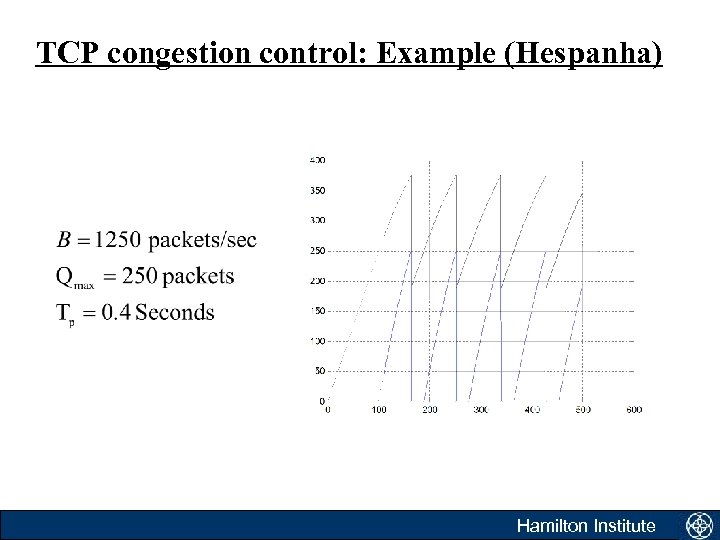
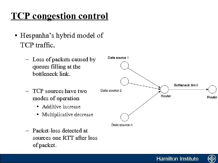TCP congestion control • Hespanha’s hybrid model of TCP traffic. – Loss of packets caused by queues filling at the bottleneck link. – TCP sources have two modes of operation • Additive increase • Multiplicative decrease – Packet-loss detected at sources one RTT after loss of packet. Hamilton Institute

TCP congestion control Hamilton Institute

Modelling the ‘queue not full’ state • The rate at which the queue grows is easy to determine. • While the queue is not full: Hamilton Institute

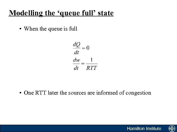Modelling the ‘queue full’ state • When the queue is full • One RTT later the sources are informed of congestion Hamilton Institute

TCP congestion control Hamilton Institute

TCP congestion control: Example (Hespanha) Hamilton Institute

TCP congestion control: Example (Fairness) Hamilton Institute