3b221054654eb94d9f212077ce1791c5.ppt
- Количество слайдов: 29


Modeling the Causes of Urban Expansion Stephen Sheppard Williams College Presentation for Lincoln Institute of Land Policy, February 16, 2006 Presentations and papers available at http: //www. williams. edu/Economics/Urban. Growth/Home. Page. htm

Urban Expansion n Urban expansion taking place world wide • Rich • Evolving from transportation choices - “car culture” • Failure of planning system? • Poor • Rural to urban migration • Urban bias? n Policy challenges • Environmental impact from transportation • Preservation of open space • Pressure for housing and infrastructure provision n Policy response • Land use planning • Public transport subsidies & private transport taxes • Rural development n n Surprisingly few global studies of this global phenomenon Limited data availability

Data To address the lack of data, we construct a sample of urban areas The sample is representative of the global urban population in cities with population over 100, 000 n Random sub-sample of UN Habitat sample n Stratified by region, city size and income level n n Urban Pop. Region Cities in 2000 Sample Population in 2000 Population Sample Cities % N % East Asia & the Pacific 410, 903, 331 550 57, 194, 979 13. 9% 16 2. 9% Europe 319, 222, 933 764 45, 147, 989 14. 1% 16 2. 1% Latin America & the Caribbean 288, 937, 443 547 70, 402, 342 24. 4% 16 2. 9% 53, 744, 935 125 22, 517, 636 41. 9% 8 6. 4% Other Developed Countries 367, 040, 756 534 77, 841, 364 21. 2% 16 3. 0% South & Central Asia 332, 207, 361 641 70, 900, 333 21. 3% 16 2. 5% Southeast Asia 110, 279, 412 260 36, 507, 583 33. 1% 12 4. 6% Sub-Saharan Africa 145, 840, 985 335 16, 733, 386 11. 5% 12 3. 6% 92, 142, 320 187 18, 360, 012 19. 9% 8 4. 3% 2, 120, 319, 475 3, 943 415, 605, 624 19. 6% 120 3. 0% Northern Africa Western Asia Total

Data – a global sample of cities Regions East Asia & the Pacific Europe Latin America & the Caribbean Northern Africa Other Developed Countries South & Central Asia Southeast Asia Sub-Saharan Africa Western Asia Population Size Class 100, 000 to 528, 000 to 1, 490, 000 and 4, 180, 000 > 4, 180, 001 Income (annual per Class capita GNP) < $3, 000 - $5, 200 - $17, 000 > $17, 000

Remote Sensing The relative brightness in different portions of the spectrum identify different types of ground cover. Satellite (Landsat TM) data measure – for pixels that are 28. 5 meters on each side – reflectance in different frequency bands

Measuring Urban Land Use 1986 Contrasting Approaches: 1. Open space within the urban area 2. Development at the urban periphery 3. Fragmented nature of development 4. Roadways in “rural” areas 2000 Earth. Sat Geocover Our Analysis

Change in urban land use

Display in Google Earth

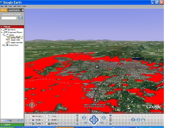
Google Earth Ground View

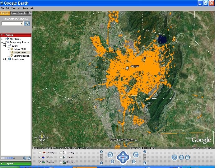
Change in urban land use: Jaipur, India

Google Earth view of Jaipur

Modeling urban land use n Households: • L households • Income y • Preferences v(c, q) • composite good c • housing q. • Household located at x pays annual transportation costs n In equilibrium, household optimization implies: for all locations x n Housing q for consumption is produced by a housing production sector
 to produce")
Modeling urban land use n Housing producers • Production function H(N, l) to produce square meters of housing • N = capital input, l=land input • Constant returns to scale and free entry determines an equilibrium land rent function r(x) and a capital-land ratio (building density) S(x) • Land value and building density decline with distance • Combining the S(x) with housing demand q(x) provides a solution for the population density D(x, t, y, u) as a function of distance t and utility level u n The extent of urban land use is determined by the condition:

Modeling urban land use n Equilibrium requires: n The model provides a solution for the extent of urban land use as a function of Population Income MP of land in housing production Transport costs n Agricultural land values Land made available for housing Generalize the model to include an export sector and obtain comparative statics with respect to: • MP of land in goods production • World price of the export good

Hypotheses Result Description 1. An increase in population will increase urban extent and urban expansion. 2. An increase in household income will increase urban extent and urban expansion. 3. An increase in transportation costs will reduce urban extent and limit urban expansion. 4. An increase in the opportunity cost of non-urban land will reduce urban extent and limit urban expansion. 5. An increase in the marginal productivity of land in housing production will cause urban expansion. 6. An increase in the share of land available for housing development will increase urban extent and urban expansion. 7. An increase in marginal productivity of land in production of the export good will increase urban extent and urban expansion. 8. An increase in the world price of the export good will increase urban extent and urban expansion.

Model estimation n We consider three classes of empirical models • Linear models of urban land cover • “Models 1 -3” • Linear models of the change in urban land cover • “Models 4 -6” • Log-linear models of urban land cover • “Models 7 -11” n Each approach has different relative merits • Linear models – simplicity and sample size • Change in urban land use – endogeneity • Log linear – interaction and capture of non-linear impact
 400.")
Linear model variables Variable Mean σ Min Max Urban Land Use (km 2) 400. 6871 533. 7343 8. 91769 2328. 87 Total Population 3, 287, 357 4, 179, 050 105, 468 1. 70 E+07 Per Capita GDP (PPP 1995 $) 9, 550. 217 9, 916. 317 562. 982 32, 636. 5 National share of IP addresses 0. 085741 0. 193696 3. 50 E-06 0. 593672 Air Linkages 88. 78808 117. 6716 0 659 Maximum Slope (percent) 25. 34515 14. 55289 4. 16 72. 78 Agricultural Rent ($/Hectare) 1, 641. 608 3, 140. 596 68. 8372 19, 442. 1 Cost of fuel ($/liter) 0. 581498 0. 328673 0. 02 1. 56 Cars per 1000 persons 144. 7495 191. 4476 0. 39 558. 5 Ground Water (1=shallow aquifer) 0. 281518 0. 451022 0 1 Temperate Humid Climate 0. 077395 0. 267979 0 1 Mediterranean Warm Climate 0. 005109 0. 071499 0 1 Mediterranean Cold Climate 0. 017234 0. 130515 0 1 Sampling Weight 0. 011168 0. 010542 0. 000834 0. 068174

Linear model estimates Variable Model 1 Model 2 Model 3 Population 0. 000077 0. 000075 0. 000073 0. 0295 0. 0355 0. 0260 IP Share 529. 3747 606. 6442 639. 3068 Air Link 0. 3207 0. 3633 0. 4040 Maximum Slope -0. 7247 -0. 3551 -0. 8658 Agricultural Rent -0. 0182 -0. 0207 -0. 0190 Income Fuel Cost 64. 0541 Cars/1000 Shallow Ground Water Fixed Effects -0. 4750 83. 5832 85. 3899 82. 3103 Biome

Models of change in urban land Variable Mean σ Min Max Change in Built-Up Area 125. 8202 163. 3169 -322. 559 527. 368 Change in Total Population 751827. 3 1474634 -470586 5. 40 E+06 Change in Per Capita GDP 1566. 28 2156. 812 -4552. 33 6722. 88 Air Links in 1990 88. 03663 124. 1801 0 659 Maximum Slope in 1990 25. 03812 14. 3309 4. 16 70. 63 Agricultural Rent in 1990 1589. 797 3396. 454 84. 9003 19442. 1 Fuel Cost in 1990 0. 436883 0. 247924 0. 02 1. 18 Cars per 1000 in 1990 130. 7622 182. 7599 0. 39 489. 2 Sampling Weight 0. 011168 0. 010573 0. 000834 0. 068174

Change in urban land model estimates Model 4 Population Change Model 5 Model 6 0. 000083 0. 000085 0. 000084 0. 02169 0. 01813 0. 020129 IP Share 237. 1614 279. 7229 270. 6102 T 1 Airlink 0. 1383 0. 1154 0. 1301 T 1 Maximum Slope -1. 2954 -1. 1688 -1. 2267 T 1 Agricultural Rent -0. 0011 Income Change T 1 Fuel Cost 21. 0234 T 1 Cars/1, 000 -0. 0199 Shallow Ground Water 36. 0570 35. 8025 36. 5591 Constant 24. 2468 10. 6364 20. 8378 Biome 88 90 90 R-squared 0. 8207 0. 816 0. 8154 Root MSE 73. 515 74. 035 74. 154 Fixed Effects Number of observations
 5. 2177 1. 3024 64")
Log-linear models Variable Mean σ Min Max Ln(Urban Area) 5. 2177 1. 3024 64 09 2. 1880 7. 7531 4 4 Ln(Total Population ) 14. 260 1. 2439 64 01 11. 566 16. 668 2 2 Ln(Per Capita GDP) 8. 5965 1. 0997 82 58 6. 3332 10. 393 5 2 5. 2 49 60 3. 0121 7 59 0. 52 14 3 Ln(Share IP Addresses) 12. 55 92 Ln(Air Links+1) 2. 9235 2. 2134 13 1 6. 4922 0 4 Ln(Maximum Slope) 3. 0657 0. 5955 46 72 1. 4255 4. 2874 2 4 Ln(Agricultura l Rent) 6. 7574 0. 9805 74 55 4. 2317 4 9. 8752 - -

Log-linear models Model 7 Model 8 Population 0. 7412 0. 7667 0. 8040 0. 7453 0. 7919 Income 0. 5674 0. 6166 0. 0707 0. 5552 0. 0931 -0. 0364 -0. 0261 -0. 0219 -0. 0220 0. 0880 0. 0754 0. 0385 0. 0790 0. 0431 Maximum Slope -0. 0568 -0. 0492 -0. 1127 -0. 0519 -0. 1074 Agricultural Rent -0. 2323 -0. 2578 -0. 2069 -0. 2693 -0. 2165 0. 1670 0. 0680 IP Share Air Links Model 9 Model 10 Model 11 Fuel Cost Cars/1000 0. 2907 0. 2671 Shallow Ground Water 0. 2920 0. 2729 0. 2183 0. 2600 0. 2163 Fixed Effects Biome Biome Note: all variables except Ground Water enter as natural log

Hypotheses tested Expected Result of Test 1. Strongly confirmed – doubling population increases urban land cover by 74 to 80 percent. 2. Confirmed – doubling national income increases urban land use by 55 to 60 percent – further investigation warranted on income and transport mode 3. Unclear – increasing fuel cost associated with increased urban land use; doubling cars per capita increases urban land use by about 26 to 29 percent in log-linear model, but decreases urban expansion in linear model – colinearity and endogeneity? 4. Strongly confirmed – doubling the value added per hectare in agriculture decreases urban land use by 20 to 26 percent 5. Confirmed – less steeply sloped land easy access to well water increases urban land use in all models 6. Confirmed – less steeply sloped land increases the share of urban land available for development and increases urban land use 7. 8. Confirmed – increased accessibility to global markets increases urban land use in all models – doubling the share of global IP addresses increases urban land use in linear and differenced models – increasing the number of direct international flights increases urban land use in all models

Policy Implications n Policies designed to limit urban expansion tend to focus on a few variables • Transportation costs and modal choice • Combat “car culture” • Provide mass transit alternatives • Limit road building • Rural to urban migration and population growth • Enhance economic opportunity in rural areas • Residence permits for cities Considerable urban expansion occurs naturally as a result of economic growth n Limiting migration could be effective but. . . n • Economic misallocation costs • Problems where free mobility considered an important right Land use planning policies? n Land taxation? n

Need for improved data n To improve model estimates tests we require more data n Field researchers • • Local planning data Local taxation data House prices and land values Transport congestion and fuel prices n Income data at local level • Big problem – explore alternative data sources

Conclusions and future directions n Continuing progress • Field research to collect data on planning policies, taxes, housing conditions and prices • Evaluation of classification accuracy • Separate modeling of infill versus peripheral expansion • Modeling at micro-scale – • transition from non-urban to urban state • Interaction with nearby local development

Conclusions and future directions n Issues to address going forward • Endogeneity issues • Income • Transport costs • Links to global economy • • n Effect of planning and tax policies Impact on housing conditions and affordability Availability of housing finance Evaluation of impacts of urban expansion With global data we are developing a deeper understanding of the urban expansion that affects virtually every local area
3b221054654eb94d9f212077ce1791c5.ppt