8c762696ba9766be6e7d36ae2865dde2.ppt
- Количество слайдов: 29
Modeling TCP in Small-Buffer Networks Mark Shifrin and Isaac Keslassy Technion (Israel)

Problem How much buffering do routers need?
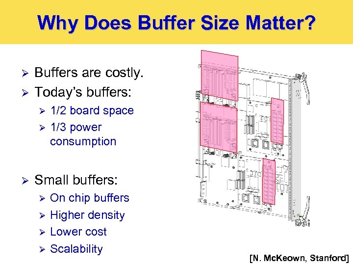
Why Does Buffer Size Matter? Ø Ø Buffers are costly. Today’s buffers: Ø Ø Ø 1/2 board space 1/3 power consumption Small buffers: Ø Ø On chip buffers Higher density Lower cost Scalability [N. Mc. Keown, Stanford]
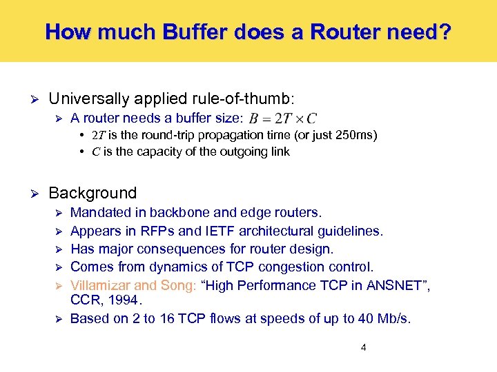
How much Buffer does a Router need? Ø Universally applied rule-of-thumb: Ø A router needs a buffer size: • 2 T is the round-trip propagation time (or just 250 ms) • C is the capacity of the outgoing link Ø Background Ø Ø Ø Mandated in backbone and edge routers. Appears in RFPs and IETF architectural guidelines. Has major consequences for router design. Comes from dynamics of TCP congestion control. Villamizar and Song: “High Performance TCP in ANSNET”, CCR, 1994. Based on 2 to 16 TCP flows at speeds of up to 40 Mb/s. 4
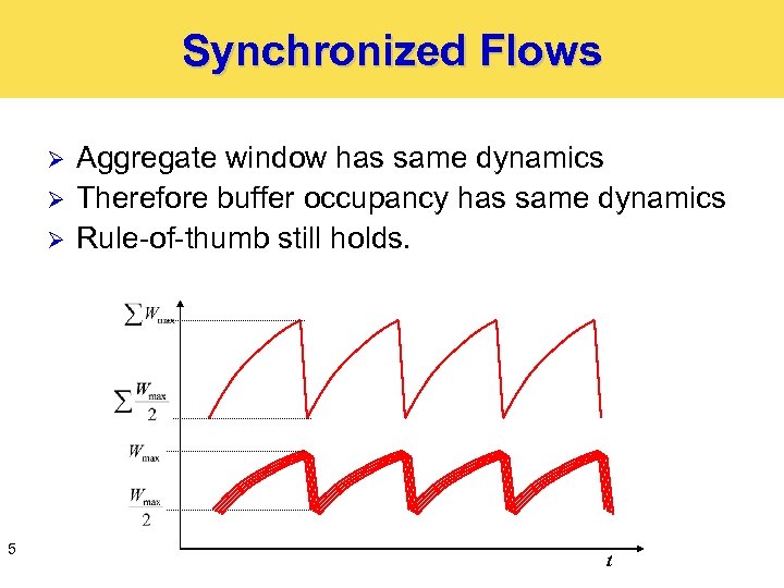
Synchronized Flows Ø Ø Ø 5 Aggregate window has same dynamics Therefore buffer occupancy has same dynamics Rule-of-thumb still holds. t
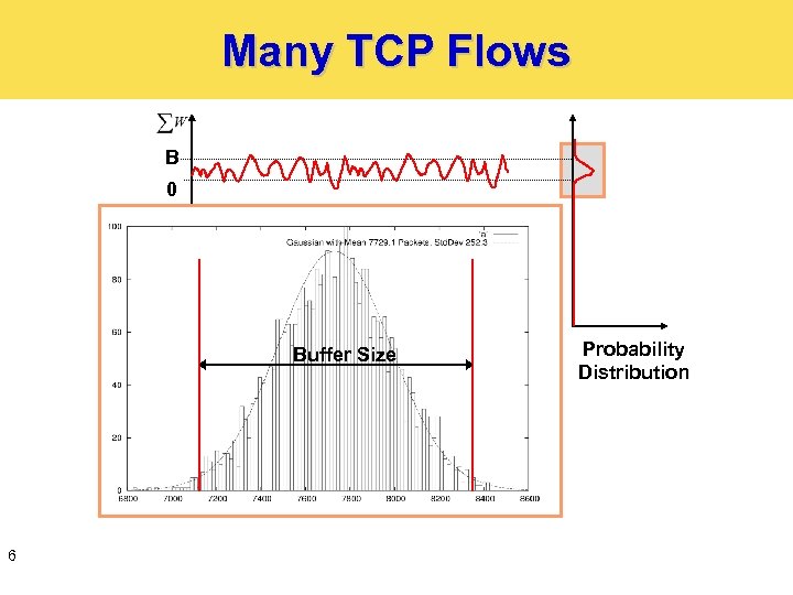
Many TCP Flows B 0 Buffer Size 6 Probability Distribution
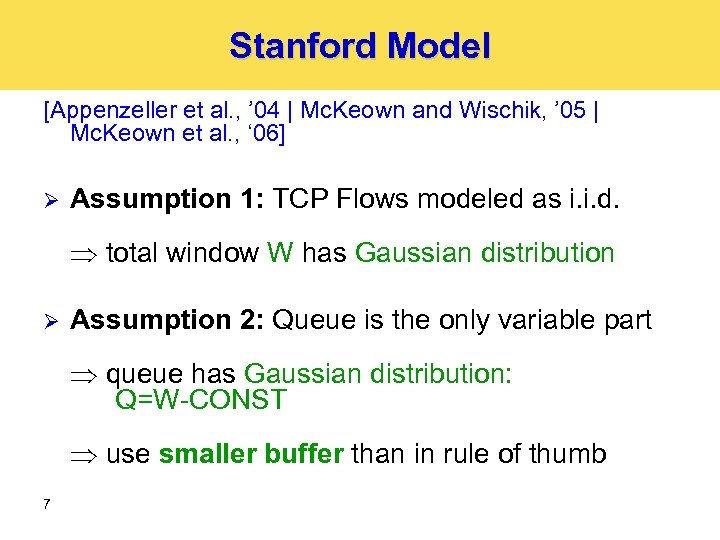
Stanford Model [Appenzeller et al. , ’ 04 | Mc. Keown and Wischik, ’ 05 | Mc. Keown et al. , ‘ 06] Ø Assumption 1: TCP Flows modeled as i. i. d. total window W has Gaussian distribution Ø Assumption 2: Queue is the only variable part queue has Gaussian distribution: Q=W-CONST use smaller buffer than in rule of thumb 7
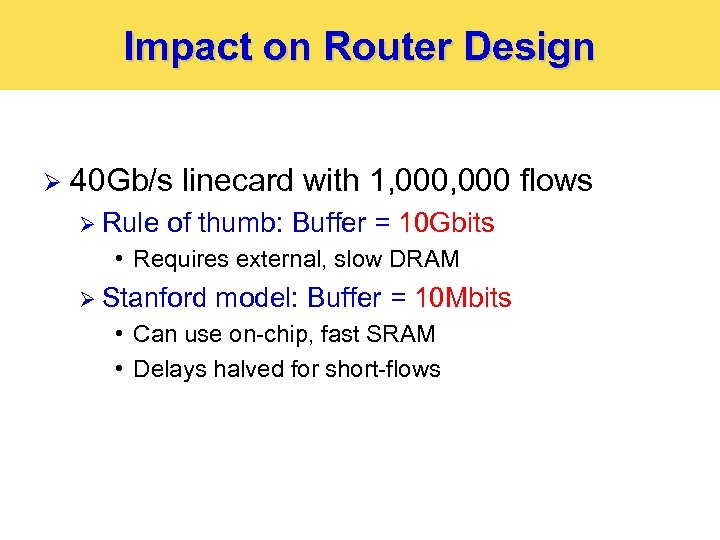
Impact on Router Design Ø 40 Gb/s linecard with 1, 000 flows Ø Rule of thumb: Buffer = 10 Gbits • Requires external, slow DRAM Ø Stanford model: Buffer = 10 Mbits • Can use on-chip, fast SRAM • Delays halved for short-flows
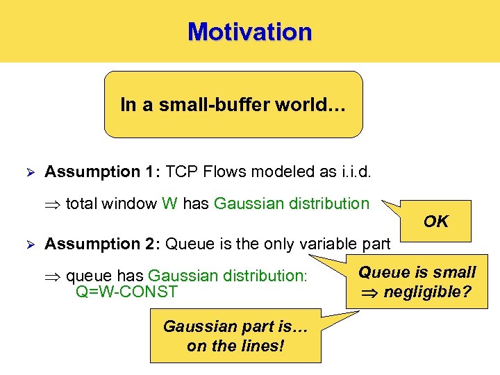
Motivation In a small-buffer world… Ø Assumption 1: TCP Flows modeled as i. i. d. total window W has Gaussian distribution Ø OK Assumption 2: Queue is the only variable part queue has Gaussian distribution: Q=W-CONST Gaussian part is… on the lines! Queue is small negligible?
Contributions Ø Distribution models for: Ø Lines Ø Arrival rates to queues Ø Queue sizes Ø Packet loss rates General closed-loop model for small-buffer networks Ø Result: queues are not the only variable part in the network Ø
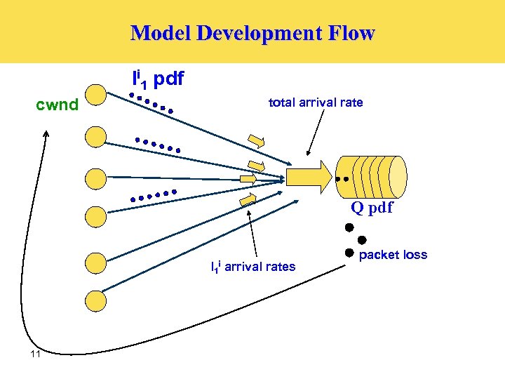
Model Development Flow li 1 pdf total arrival rate cwnd Q pdf l 1 arrival rates i 11 packet loss
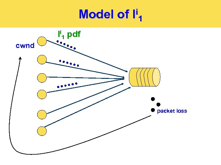
Model of li 1 pdf cwnd packet loss
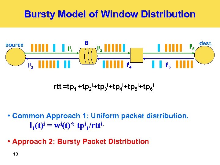
Bursty Model of Window Distribution source li 1 B li 5 li 3 li 4 li 2 li 6 rtti=tp 1 i+tp 2 i+tp 3 i+tp 4 i+tp 5 i+tp 6 i • Common Approach 1: Uniform packet distribution. l 1(t)i = wi(t)* tpi 1/rtti. • Approach 2: Bursty Packet Distribution 13 dest.
Bursty Model of Window Distribution Ø Assumption: All packets in a flow move in a single burst Ø Conclusion 1: All packets belonging to an arbitrary flow i are present almost always on the same link. Ø Conclusion 2: The probability of burst of flow i being present on the certain link is equal to the ratio of its propagation latency to the total rtti. 14
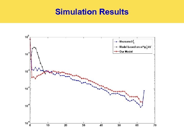
Simulation Results 15
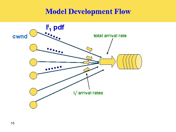
Model Development Flow li 1 pdf cwnd total arrival rate l 1 i arrival rates 16
Rate Transmission Derivation Ø Ø The objective is to find the pdf of the number of packets sent on some link i, ri, in a time unit δt. Assumptions: Ø Ø Ø 17 The rate on each one of the links in L 1 is statistically independent We assume that the transmissions are bursty. We assume that the rate is proportional to the distribution of l 1 i and to the ratio δt/tp 1 i.
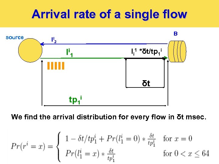
Arrival rate of a single flow source B li 2 l i 1 li 1 *δt/tp 1 i δt tp 1 i We find the arrival distribution for every flow in δt msec.
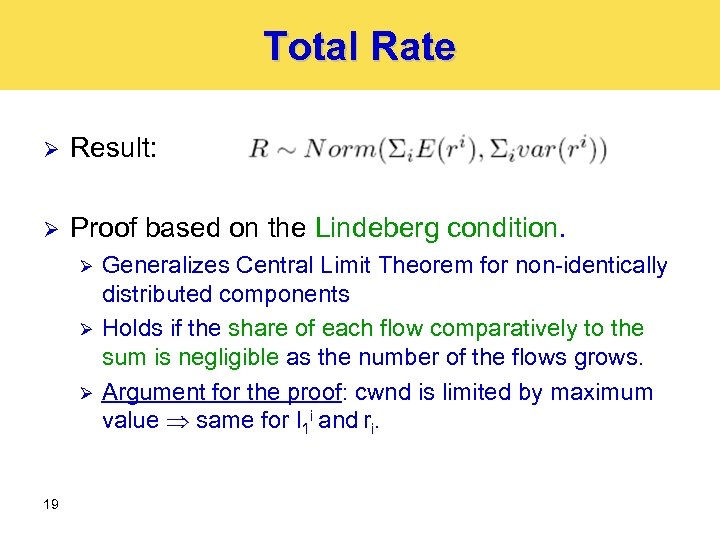
Total Rate Ø Result: Ø Proof based on the Lindeberg condition. Ø Ø Ø 19 Generalizes Central Limit Theorem for non-identically distributed components Holds if the share of each flow comparatively to the sum is negligible as the number of the flows grows. Argument for the proof: cwnd is limited by maximum value same for l 1 i and ri.
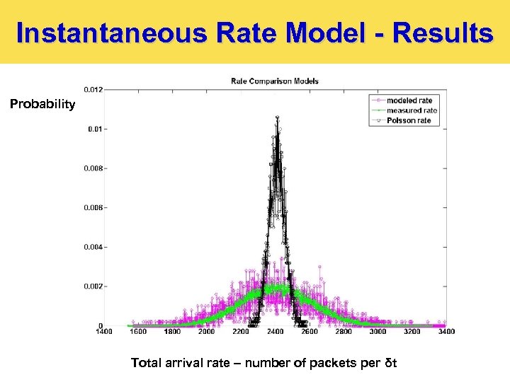
Instantaneous Rate Model - Results Probability Total arrival rate – number of packets per δt
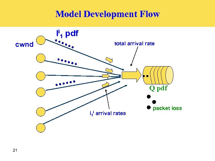
Model Development Flow li 1 pdf total arrival rate cwnd Q pdf l 1 arrival rates i 21 packet loss
PDF for Q Ø To find the queue size distribution: Ø Run Markov Chain simulation (compared with [Tran-Gia and Ahmadi, ‘ 88]) Ø Use samples of R for the transitions Ø 22 Packet loss p is derived from the queue size distribution.
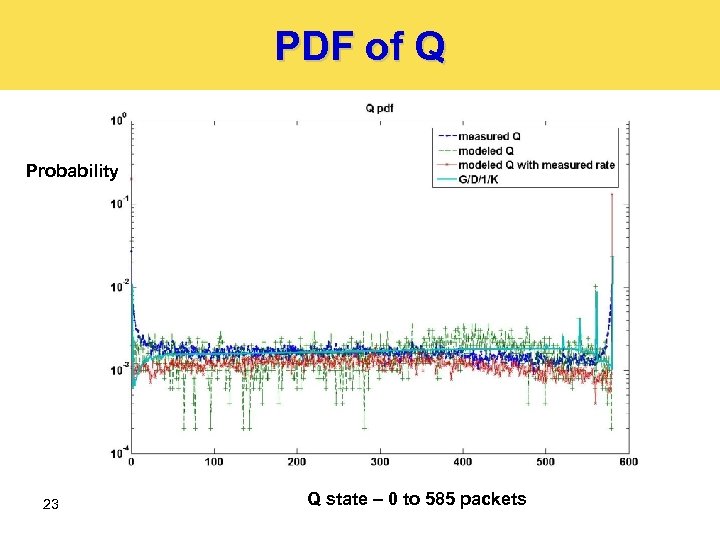
PDF of Q Probability 23 Q state – 0 to 585 packets
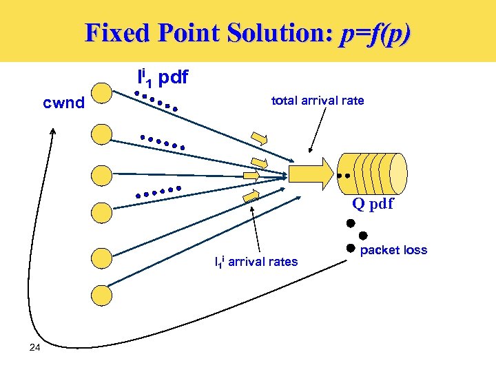
Fixed Point Solution: p=f(p) li 1 pdf total arrival rate cwnd Q pdf l 1 arrival rates i 24 packet loss
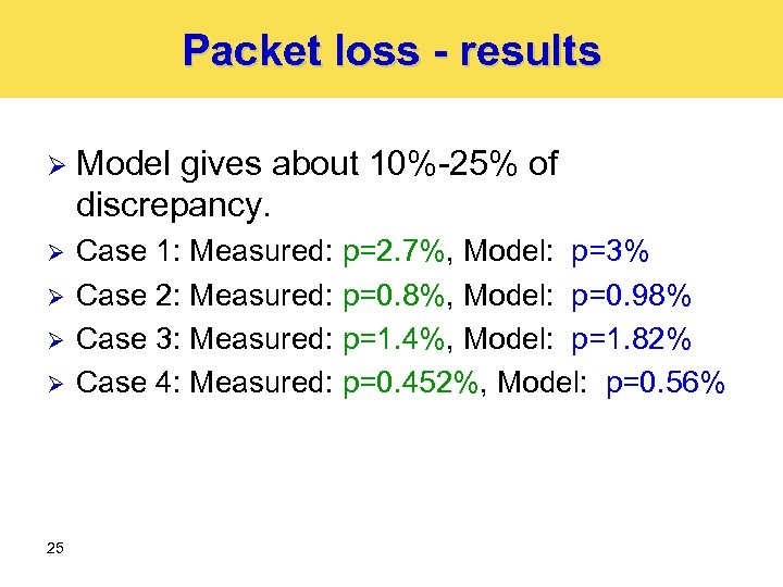
Packet loss - results Ø Model gives about 10%-25% of discrepancy. Ø Case 1: Measured: p=2. 7%, Model: p=3% Case 2: Measured: p=0. 8%, Model: p=0. 98% Case 3: Measured: p=1. 4%, Model: p=1. 82% Case 4: Measured: p=0. 452%, Model: p=0. 56% Ø Ø Ø 25
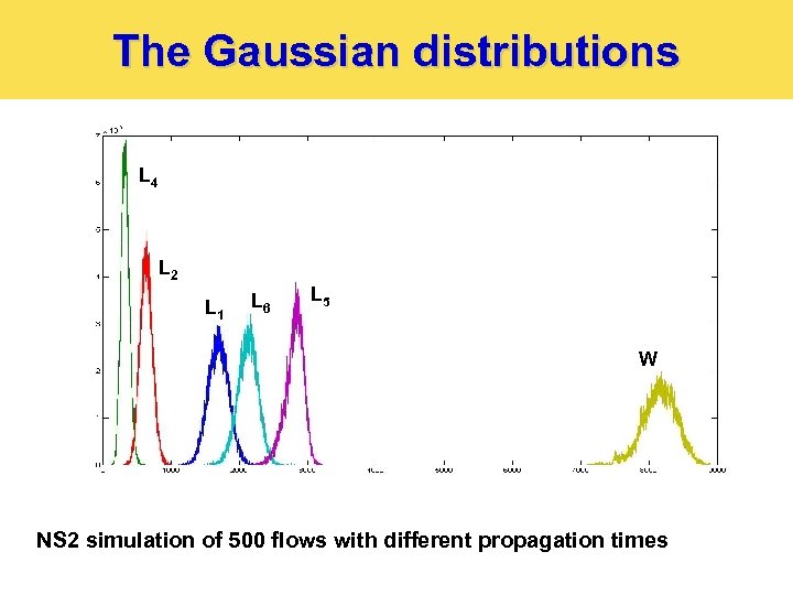
The Gaussian distributions L 4 L 2 L 1 L 6 L 5 W NS 2 simulation of 500 flows with different propagation times
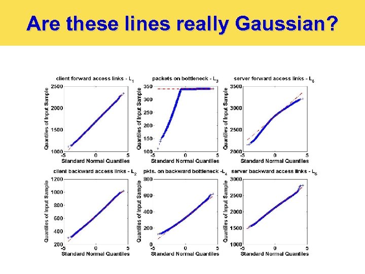
Are these lines really Gaussian? 27
Summary Ø Introduced general closed-loop model for small-buffer networks Ø Proved wrong the usual assumption that queues are the only variable part in the network 28

Thank you.
8c762696ba9766be6e7d36ae2865dde2.ppt