Modeling Overview for LTCP Development Julia Moore P

Modeling Overview for LTCP Development Julia Moore, P. E. Limno-Tech, Inc.

Items to Be Covered Modeling and the CSO Control Policy Combined sewer system (CSS) modeling Receiving water (RW) modeling Model review 2 Modeling Overview

Expectations of the CSO Policy EPA supports the proper and effective use of models, where appropriate, in the evaluation of the nine-minimum controls and the development of the long-term control plan… Resource – Combined Sewer Overflows: Guidance for Monitoring and Modeling. EPA 832 B-99 -002. January, 1999. 3 Modeling Overview

Expectations of the CSO Policy Event modeling The permittee should adequately characterize through monitoring, modeling, and other means as appropriate, for a range of storm events, the response of its sewer system to wet weather events… Section II. C. 1 Continuous simulation modeling EPA believes that continuous simulation models, using historical rainfall data, may be the best way to model sewer systems, CSOs, and their impacts… Section II. C. 1. d 4 Modeling Overview

Why is CSS Modeling Important? Good characterization is typically infeasible without models except for small / simple systems “Stretch” the value of monitoring, saving time and money Assess conveyance and storage for NMC and LTCP Optimize LTCP under a range of storm conditions Provide a tool for projecting results after implementation of CSO controls 5 Modeling Overview

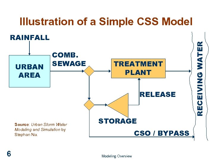RAINFALL URBAN AREA COMB. SEWAGE TREATMENT PLANT RELEASE Source: Urban Storm Water Modeling and Simulation by Stephan Nix 6 STORAGE CSO / BYPASS Modeling Overview RECEIVING WATER Illustration of a Simple CSS Model

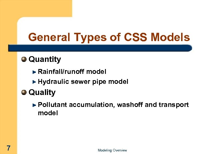General Types of CSS Models Quantity Rainfall/runoff model Hydraulic sewer pipe model Quality Pollutant accumulation, washoff and transport model 7 Modeling Overview

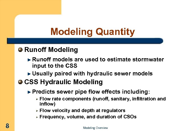Modeling Quantity Runoff Modeling Runoff models are used to estimate stormwater input to the CSS Usually paired with hydraulic sewer models CSS Hydraulic Modeling Predicts sewer pipe flow effects including: Flow rate components (runoff, sanitary, infiltration and inflow) Flow velocity and depth at regulators Frequency, volume, and duration of CSOs 8 Modeling Overview

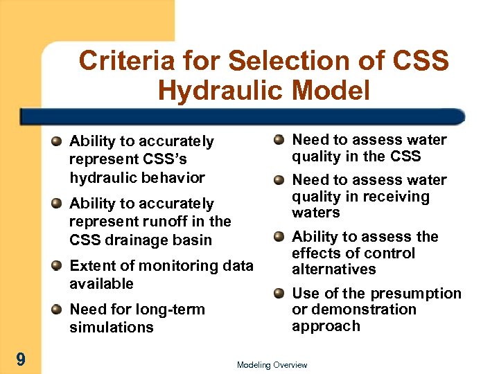Criteria for Selection of CSS Hydraulic Model Need to assess water quality in the CSS Ability to accurately represent CSS’s hydraulic behavior Need to assess water quality in receiving waters Ability to accurately represent runoff in the CSS drainage basin Extent of monitoring data available Need for long-term simulations 9 Ability to assess the effects of control alternatives Use of the presumption or demonstration approach Modeling Overview

Model Complexity Levels of detail Coarse (e. g. , STORM) Simplified sewer network Lumped parameter Moderate (e. g. , SWMM/TRANSPORT) Major pipes/interceptors only Unable to simulate complex flow (e. g. , backwater conditions, tidal influence) Fine (e. g. , SWWM/EXTRAN, MOUSE) All major sewer components (storage, pumping, and smaller diameter pipes) Able to simulate complex flow 10 Modeling Overview

Level of Detail Selection of Appropriate Level Identify benefits from a finer level of detail Consider penalties (accuracy) in not modeling a portion of the system Adopt a staged approach - start from simple model and build complexity as needed and as data become available. 11 Modeling Overview

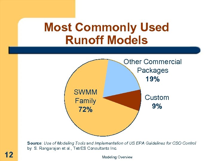Most Commonly Used Runoff Models Other Commercial Packages 19% SWMM Family 72% 12 Custom 9% Source: Use of Modeling Tools and Implementation of US EPA Guidelines for CSO Control by S. Rangarajan et al. , Tetr. ES Consultants Inc. Modeling Overview

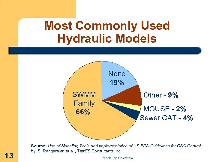Most Commonly Used Hydraulic Models None 19% SWMM Family 66% 13 Other - 9% MOUSE - 2% Sewer CAT - 4% Source: Use of Modeling Tools and Implementation of US EPA Guidelines for CSO Control by S. Rangarajan et al. , Tetr. ES Consultants Inc. Modeling Overview

Calibration Data Need range of typical storm events 3 to 5 storms (minimum) Small (0. 1 -0. 4”), medium (0. 4 -1. 0”) to large (>1. 0”) storms Individual storm events (return to dry weather) Measure Ø Rainfall (hourly data; multiple locations) Ø Overflow volume Ø Effluent quality (for input to receiving water model) 14 Modeling Overview

Data Review Flow monitoring data Consistent with rainfall data Manning’s Equation (calculate velocity, flow and depth) Flow balance review (downstream flows are consistent with upstream flows) Outfall quality data 15 Can be highly variable Compare to influent data/literature Compare to other outfall data Modeling Overview

Model Development Develop pipe network Establish operational rules for hydraulic controls Estimate dry weather component of flow Conduct initial testing of model Conduct model sensitivities Guides calibration Modify model parameters by +/- 25% to assess sensitivity 16 Modeling Overview

Calibration Methods, Tools Calibration process, sequence – volume, peaks/timing, pollutants Graphical depictions of quality of fit – hydrograph plots, 1: 1 plots Measures of quality of fit – RMS error, SSD, sum of absolute differences 17 Modeling Overview

Calibration Methods, Tools Statistical comparisons of volumes and peak flows Range of storms +/- 20% modeled versus observed Avoid bias Source: Urban Stormwater Modeling and Simulation by Stephan Nix 18 Modeling Overview

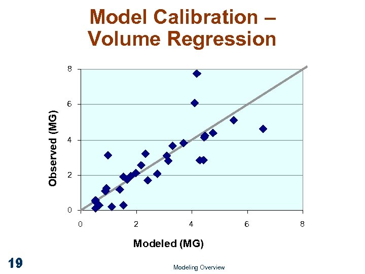Model Calibration – Volume Regression 8 Observed (MG) 6 4 2 0 0 2 4 Modeled (MG) 19 Modeling Overview 6 8

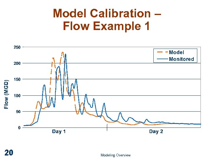Model Calibration – Flow Example 1 20 Modeling Overview

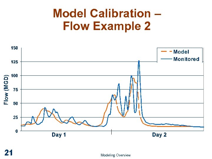Model Calibration – Flow Example 2 21 Modeling Overview

Why is RW Modeling Important? Characterize the RW impacts under different CSO loads and conditions Discern contributions of background and other sources Predict benefits of CSO alternatives Demonstrate WQ standards attainment or the need for a TMDL or UAA 22 Modeling Overview

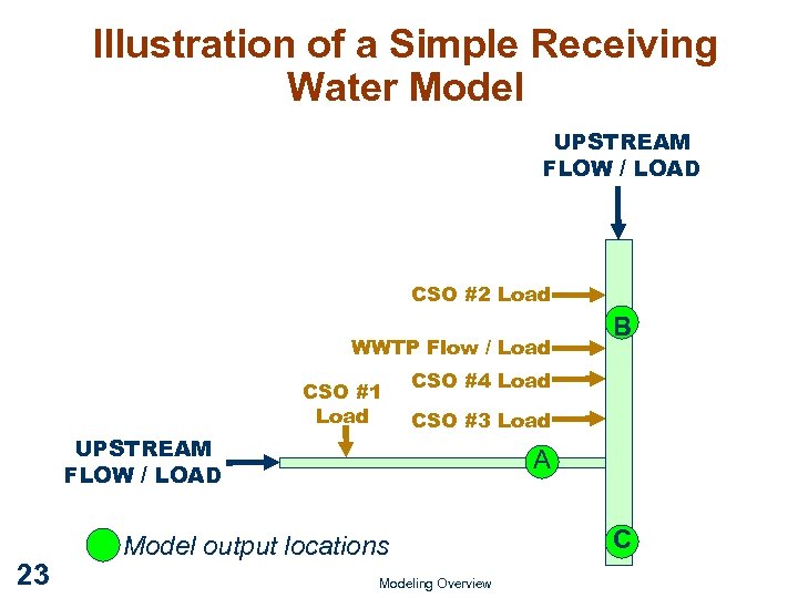Illustration of a Simple Receiving Water Model UPSTREAM FLOW / LOAD CSO #2 Load WWTP Flow / Load CSO #1 Load UPSTREAM FLOW / LOAD 23 B CSO #4 Load CSO #3 Load A Model output locations Modeling Overview C

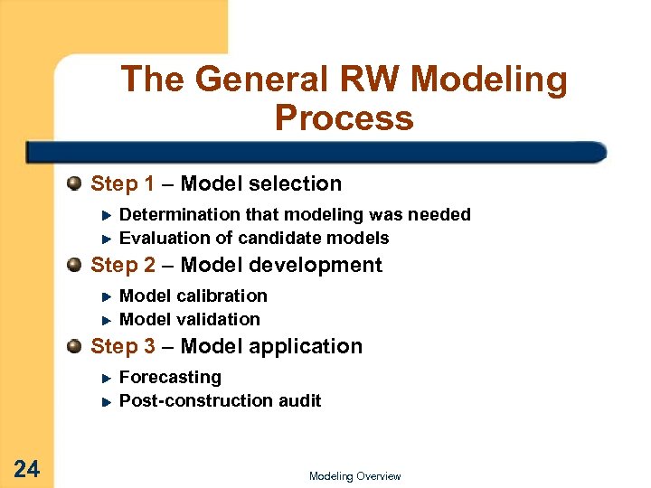The General RW Modeling Process Step 1 – Model selection Determination that modeling was needed Evaluation of candidate models Step 2 – Model development Model calibration Model validation Step 3 – Model application Forecasting Post-construction audit 24 Modeling Overview

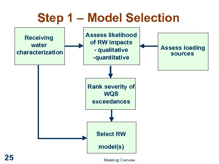Step 1 – Model Selection Receiving water characterization Assess likelihood of RW impacts - qualitative -quantitative Rank severity of WQS exceedances Select RW model(s) 25 Modeling Overview Assess loading sources

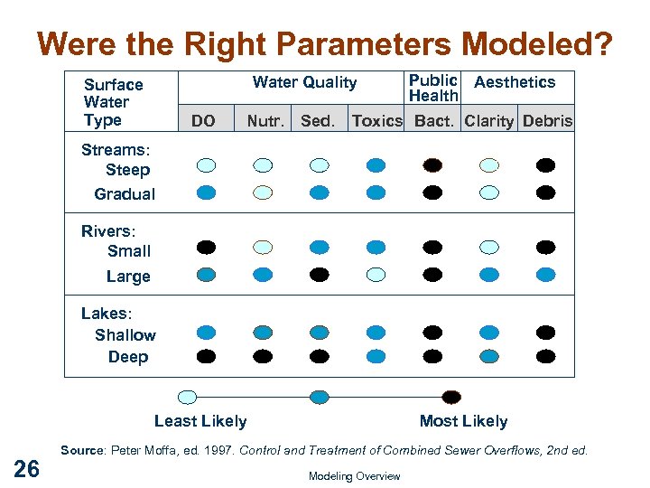Were the Right Parameters Modeled? Water Quality Surface Water Type DO Nutr. Sed. Public Aesthetics Health Toxics Bact. Clarity Debris Streams: Steep Gradual Rivers: Small Large Lakes: Shallow Deep Least Likely 26 Most Likely Source: Peter Moffa, ed. 1997. Control and Treatment of Combined Sewer Overflows, 2 nd ed. Modeling Overview

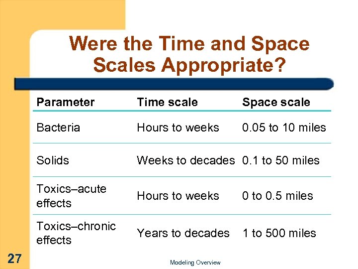Were the Time and Space Scales Appropriate? Parameter Space scale Bacteria Hours to weeks 0. 05 to 10 miles Solids Weeks to decades 0. 1 to 50 miles Toxics–acute effects Hours to weeks 0 to 0. 5 miles Toxics–chronic effects 27 Time scale Years to decades 1 to 500 miles Modeling Overview

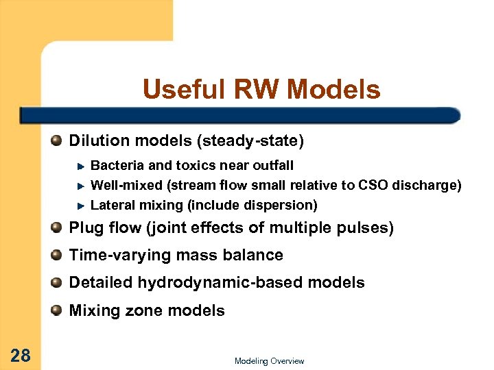Useful RW Models Dilution models (steady-state) Bacteria and toxics near outfall Well-mixed (stream flow small relative to CSO discharge) Lateral mixing (include dispersion) Plug flow (joint effects of multiple pulses) Time-varying mass balance Detailed hydrodynamic-based models Mixing zone models 28 Modeling Overview

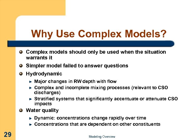Why Use Complex Models? Complex models should only be used when the situation warrants it Simpler model failed to answer questions Hydrodynamic Major changes in RW depth with flow Complex and incomplete mixing processes (relevant to CSO discharges) Stratified systems that significantly accentuate or attenuate CSO impacts Water quality Dynamic: concentrations change rapidly over time Concentrations that are dependent on other constituents 29 Modeling Overview

Step 2 – Model Development Are all significant pollutant sources (or loss mechanisms) included? Are the estimates of discharge volumes and concentrations reasonable? Do the model input rates fall within accepted values? Do the model results compare with observed data? 30 Modeling Overview

Two Methods of Calibration Subjective: visual comparison of simulation with data Often uses additional information Best option when working with multiple state variables Employs modeler’s intuition in the process Objective: quantitative measure of quality of fit (usually minimize error) Not necessarily better Make sure kinetic coefficients end up within reasonable range 31 Modeling Overview

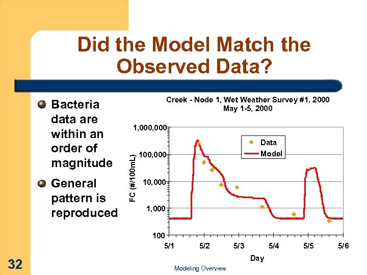Did the Model Match the Observed Data? General pattern is reproduced Creek - Node 1, Wet Weather Survey #1, 2000 May 1 -5, 2000 1, 000 FC (#/100 m. L) Bacteria data are within an order of magnitude Data Model 100, 000 1, 000 100 5/1 32 5/3 5/4 Day Modeling Overview 5/5 5/6

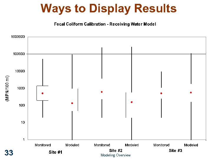Ways to Display Results 33 Modeling Overview

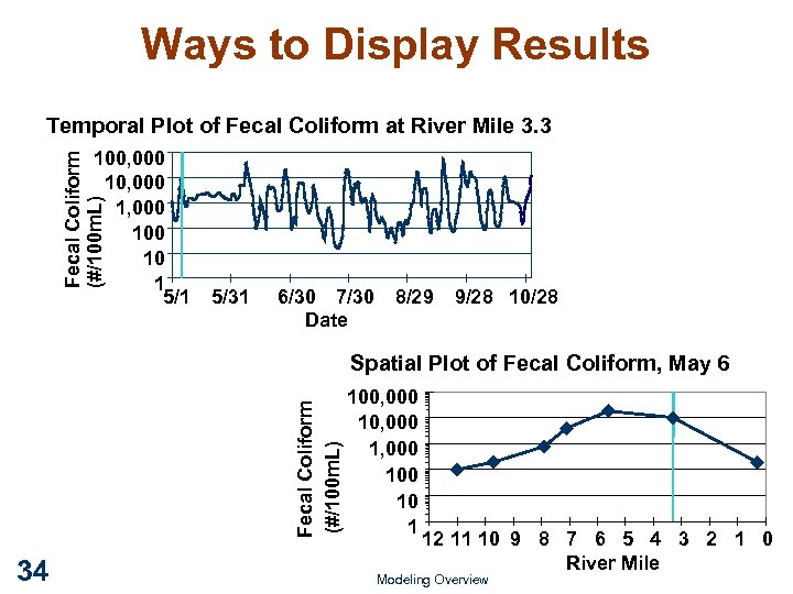Ways to Display Results Temporal Plot of Fecal Coliform at River Mile 3. 3 Fecal Coliform (#/100 m. L) 100, 000 1, 000 10 1 5/31 6/30 7/30 Date 8/29 9/28 10/28 Fecal Coliform (#/100 m. L) Spatial Plot of Fecal Coliform, May 6 34 100, 000 1, 000 10 1 12 11 10 9 8 7 6 5 4 3 2 1 0 River Mile Modeling Overview

Methods for Validation A RW model should not be considered truly “calibrated” until the model is tested over a wide range of conditions, produces explainable results, and is validated. 35 Independent data set Sensitivity analyses Component analysis Addition of synthetic loads to identify unmodeled sources Modeling Overview

Model Validation With Independent Data Demonstrates the model is capable of simulating a wider range of conditions The model is run with same rates but different loads and environmental conditions that correspond to: An event from historical data Another event from the CSO monitoring program Data collected in the future as part of the continuing planning process 36 Modeling Overview

Questions for the LTCP Reviewer to Answer Were the data sufficient to develop a reliable model? Was the selected model suitable for assessing the extent of CSO impacts? Was the model suitable for distinguishing impacts from different sources? Did the application exceed the known limitations of the model? 37 Modeling Overview

Step 3 – Model Application Was modeling used to help select the recommended plan (watershed example and component analysis)? Did the modeling demonstrate compliance of selected plan with WQ standards? If not, did the modeling help define what is needed to comply with WQ standards? 38 Modeling Overview

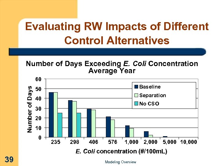Evaluating RW Impacts of Different Control Alternatives Number of Days Exceeding E. Coli Concentration Average Year Number of Days 60 Baseline 50 Separation 40 No CSO 30 20 10 0 235 298 406 576 1, 000 2, 000 5, 000 10, 000 E. Coli concentration (#/100 m. L) 39 Modeling Overview

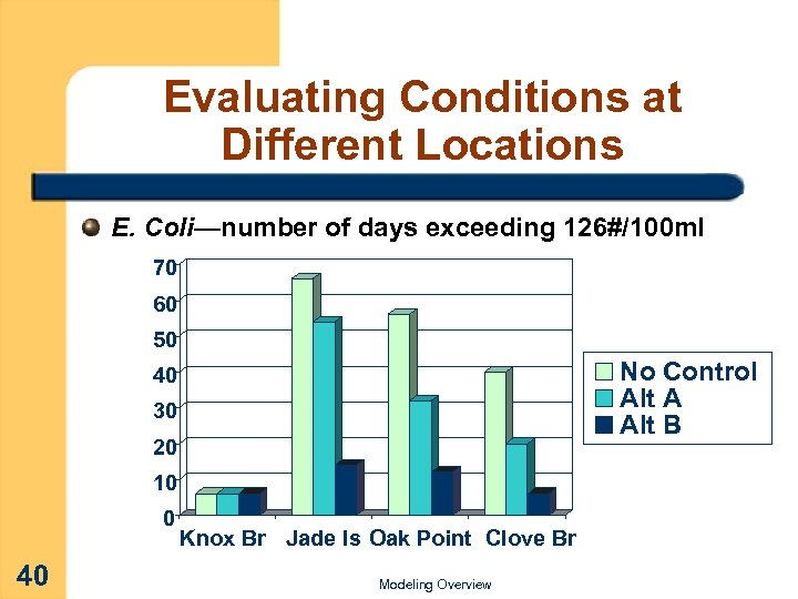Evaluating Conditions at Different Locations E. Coli—number of days exceeding 126#/100 ml 70 60 50 No Control Alt A Alt B 40 30 20 10 0 40 Knox Br Jade Is Oak Point Clove Br Modeling Overview

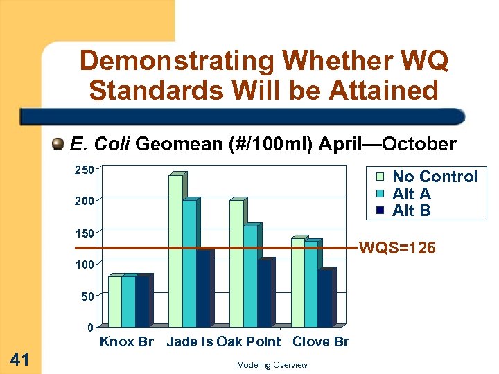Demonstrating Whether WQ Standards Will be Attained E. Coli Geomean (#/100 ml) April—October 250 No Control Alt A Alt B 200 150 WQS=126 100 50 0 41 Knox Br Jade Is Oak Point Clove Br Modeling Overview

Questions to Ask About RW Models Do modeling choices generally agree with LTCP reviewer’s expectations? What questions need to be answered? Were the right parameters modeled? Do results reflect the likely severity of impacts and benefits of control? Do the selected models fit the time scales of the anticipated problems (hourly–daily–monthly)? 42 Was the spatial coverage appropriate (impacted river miles)? Modeling Overview

Useful RW Modeling References Moffa, Peter. 1997. The Control and Treatment of Combined Sewer Overflows (2 nd Edition). Van Nostrand Reinhold, NY. EPA. 1997. Compendium of Tools for Watershed Assessment and TMDL Development. US EPA OW, Washington, DC, EPA 841 -B-97 -006. Chapra, Steven. 1997. Surface Water-Quality Modeling. Mc. Graw -Hill, NY. Thomann. Robert, Mueller, J. 1987. Principles of Surface Water Quality Modeling and Control. Harper & Rowe, NY. Bowie, et al. 1985. Rates, Constants, and Kinetics Formulations in Surface Water Quality Modeling (2 nd Edition). US EPA ORD, Athens, GA, EPA/600/3 -85/040. 43 Modeling Overview

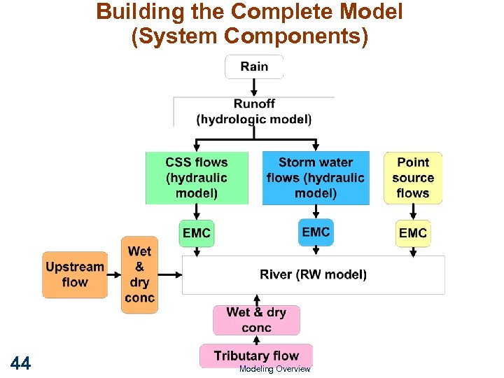Building the Complete Model (System Components) 44 Modeling Overview

Review Philosophy Reality There is never “enough” data & information All models are imperfect representations—some better than others You can’t double-check everything So what’s an LTCP reviewer to do? Adopt realistic review goals Begin with the “end-in-mind” 45 Modeling Overview

Review Approach Adopt realistic review goals Look for congruency & consistency (does it all hang together well? ) Check that level of complexity was appropriate Identify any fatal flaws and deficiencies Check that all the policy “i”s are dotted and “t”s crossed (use a checklist) Be cautious of “black box” software Begin review with the “end-in-mind” 46 Different models handle certain controls better Hindsight is 20/20–could model and calibration choices be driving critical LTCP decisions? Modeling Overview

Getting Ready What “end-in-mind” questions need to be answered during the review? What models are well suited and how should they be calibrated forecasting benefits of selected alternatives? Are the model results used appropriately in alternatives analysis? For example, a model framework oriented and calibrated for peak flow rates, then applied to single design storm events may not work for assessing the benefits of a storage control alternative. 47 Modeling Overview

Some Common Modeling Mistakes Excess complexity in place of sound engineering judgment Occam’s Razor principle—the simpler of two approaches is more likely to be the correct one Wasting resources on building a detailed model without answering the questions Lack of available data to support model capabilities Example—SWMM dirt accumulation/washoff; STORM firstflush routines are dangerous without data… 48 Modeling Overview

Common Modeling Mistakes (Cont. ) Automation run amok? Extra scrutiny is always warranted for: Automated and “black box” interfaces for radar rainfall, GIS information, runoff to sewer system, point source loads, and statistics output Program code that replaces judgment about model coefficients Program code that auto-designs pipe conveyance and pumping or river geometry Program code that auto-simplifies the system to reduce computation needs Questions? Seek clarification from the permittee 49 Modeling Overview

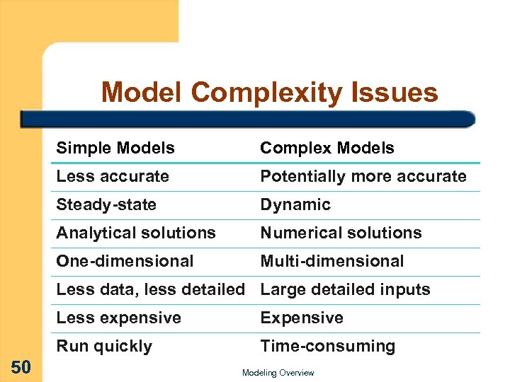Model Complexity Issues Simple Models Complex Models Less accurate Potentially more accurate Steady-state Dynamic Analytical solutions Numerical solutions One-dimensional Multi-dimensional Less data, less detailed Large detailed inputs Less expensive Run quickly 50 Expensive Time-consuming Modeling Overview

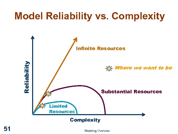Model Reliability vs. Complexity Reliability Infinite Resources Where we want to be Substantial Resources Limited Resources Complexity 51 Modeling Overview

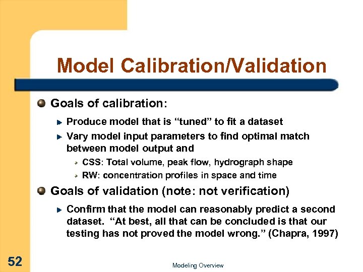Model Calibration/Validation Goals of calibration: Produce model that is “tuned” to fit a dataset Vary model input parameters to find optimal match between model output and CSS: Total volume, peak flow, hydrograph shape RW: concentration profiles in space and time Goals of validation (note: not verification) Confirm that the model can reasonably predict a second dataset. “At best, all that can be concluded is that our testing has not proved the model wrong. ” (Chapra, 1997) 52 Modeling Overview

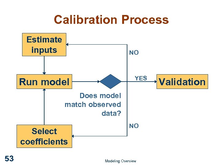Calibration Process Estimate inputs NO YES Run model Does model match observed data? Select coefficients 53 NO Modeling Overview Validation

Model Reliability and Accuracy Model predictions can be characterized in terms of reliability and accuracy: Reliability—measure of the confidence in model predictions for a specific set of conditions and for a specific confidence level Accuracy—measure of the agreement between model predictions and observations 54 Modeling Overview

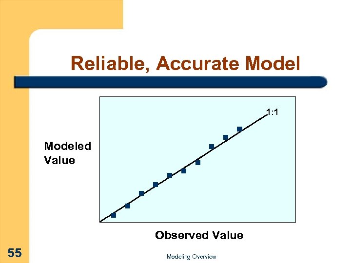Reliable, Accurate Model 1: 1 Modeled Value Observed Value 55 Modeling Overview

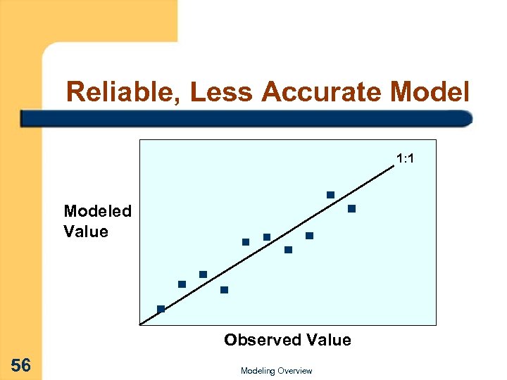Reliable, Less Accurate Model 1: 1 Modeled Value Observed Value 56 Modeling Overview

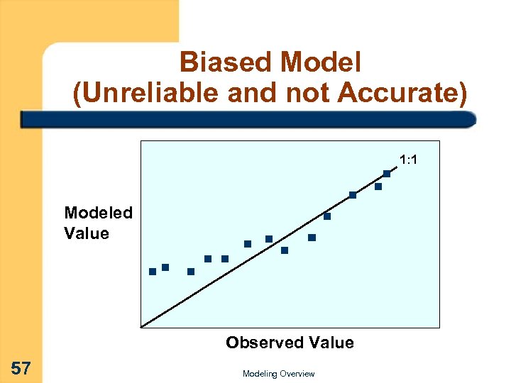Biased Model (Unreliable and not Accurate) 1: 1 Modeled Value Observed Value 57 Modeling Overview

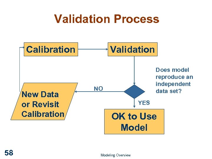Validation Process Calibration New Data or Revisit Calibration 58 Validation Does model reproduce an independent data set? NO YES OK to Use Modeling Overview

Model Validation Problems Lack of an independent data set for validation Three factors can produce unreasonable results: Poor data happens and can sometimes lead modelers astray Model may not contain sufficient detail to adequately characterize the CSS and/or RW and generate reliable output (or too complex) All models have inherent limitations and the model selected may not be adequate or poorly chosen 59 Modeling Overview

Model Application – Single Event Simulation Design storm approach Simpler to analyze and interpret (useful for initial screening) Suitable for quicker comparative analysis of control alternatives Likely to have good amount of data available on a spatial and temporal scale 60 Modeling Overview

Model Application – Continuous Simulation Used for evaluating a range of long-term CSO control alternatives Accounts for sequencing of rainfall, upstream flows, and other pollutant sources Computational speed of PCs allow simulations within a reasonable run time 61 Modeling Overview

Post-Processing of Results Often one of the largest tasks Also most important - includes: Organizing, archiving output data Plotting/visualizing data to verify quality of cal/val Porting output of CSS, etc. to RW model This is where many mistakes get made Modelers have lots of discretion in interpreting and presenting results 62 Modeling Overview

Interpretation of Results Following should be remembered Model forecasts are as accurate as user’s understanding and knowledge of system and the model. Model forecasts are no better than quality of calibration and validation and the quality of data used. Model forecasts are only estimates of the response of the CSS and RW to rainfall events. 63 Modeling Overview

Points to Remember Models are imperfect but useful tools Stretch expensive data Forecast effects of controls Important for LTCP to choose the right models to fit the situation (meets project needs without excess complexity) OK to mix and match when justified 64 Modeling Overview

Points to Remember Calibration and validation using good data are necessary for confidence in LTCP forecasts Continuous simulation is usually the best way to apply models and evaluate CSO controls; the longer the better (1 to 5 years) Understand the system and question counter-intuitive model results 65 Modeling Overview