Modeling Flows John H Vande Vate Spring 2006

Modeling Flows John H. Vande Vate Spring, 2006 1 1

New Project Opportunity • • • Sponsor: CARE and Shelter First Design temporary shelters (tents) Design delivery mechanism Design logistics network Evaluate inventory levels, locations and cost 2 2

Agenda • Network Flows – Review definition – Simple Transportation Model – Minimum Cost Flow Model • Adding Realism – – Multiple commodities Weight, Cube, Linear Cube Concave Costs Modeling Time 3 3

Reference • Network Flows: Theory, Algorithms, and Applications (Hardcover) by Ravindra K. Ahuja, Thomas L. Magnanti, James B. Orlin 4 4

What Are They? • Specially Structured Linear Programs • Each variable appears in at most two constraints – At most one constraint with a +1 coefficient – At most one constraint with a -1 coefficient • Each variable may be constrained by bounds • Integer Data => Integer Solutions 5 5

Transportation Model • • • Move Goods from Plants to Warehouses Single Commodity! Plants have supplies Warehouses have demands Costs are proportional to volume shipped (this usually isn’t very realistic) 6 6

Example 2 -3 (p 36) • Single Product • Two plants with identical production costs • Two warehouses • Markets allocated to warehouses for now • Proportional transportation costs 7 7

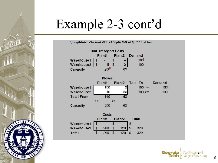Example 2 -3 cont’d 8 8

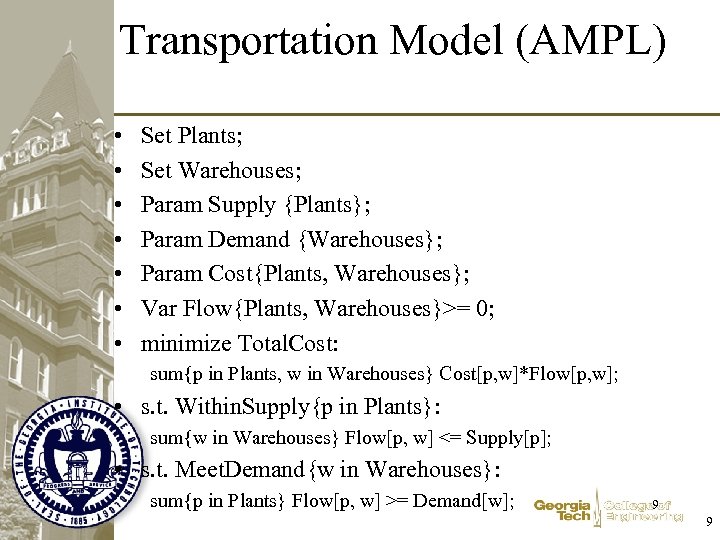Transportation Model (AMPL) • • Set Plants; Set Warehouses; Param Supply {Plants}; Param Demand {Warehouses}; Param Cost{Plants, Warehouses}; Var Flow{Plants, Warehouses}>= 0; minimize Total. Cost: sum{p in Plants, w in Warehouses} Cost[p, w]*Flow[p, w]; • s. t. Within. Supply{p in Plants}: sum{w in Warehouses} Flow[p, w] <= Supply[p]; • s. t. Meet. Demand{w in Warehouses}: sum{p in Plants} Flow[p, w] >= Demand[w]; 9 9

Minimum Cost Flow • Move Goods from Plants to Markets via Warehouses • Single Commodity! • Plants have supplies • Markets have demands • Costs are proportional to volume shipped 10 10

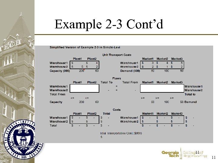Example 2 -3 Cont’d 11 11

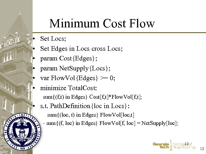Minimum Cost Flow • • • Set Locs; Set Edges in Locs cross Locs; param Cost{Edges}; param Net. Supply{Locs}; var Flow. Vol{Edges} >= 0; minimize Total. Cost: sum{(f, t) in Edges} Cost[f, t]*Flow. Vol[f, t]; • s. t. Path. Definition{loc in Locs}: sum{(loc, t) in Edges} Flow. Vol[loc, t] - sum{(f, loc) in Edges} Flow. Vol[f, loc] = Net. Supply[loc]; 12 12

Homogenous Product Must be able to interchange positions of product anywhere 13 13

Another New Project • Milliken & Co. growing business in Asia looking to explore distribution strategy: Where should it be positioning inventories to serve that region? 14 14

Multi-Commodity Flows • Several single commodity models • You can’t to turn lead into gold – Conserve flow of each product through each facility • Joined by common constraints – Often capacity on lanes – Or modeling cost (through capacity) –… 15 15

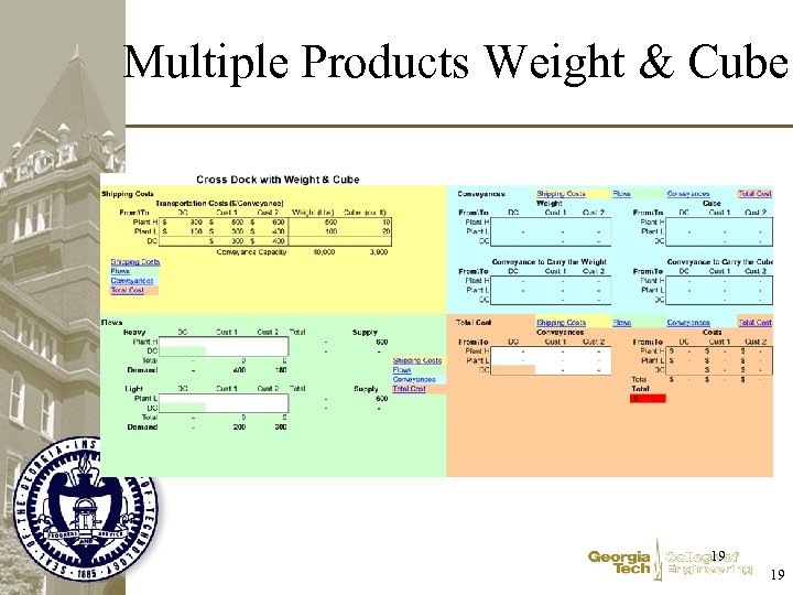
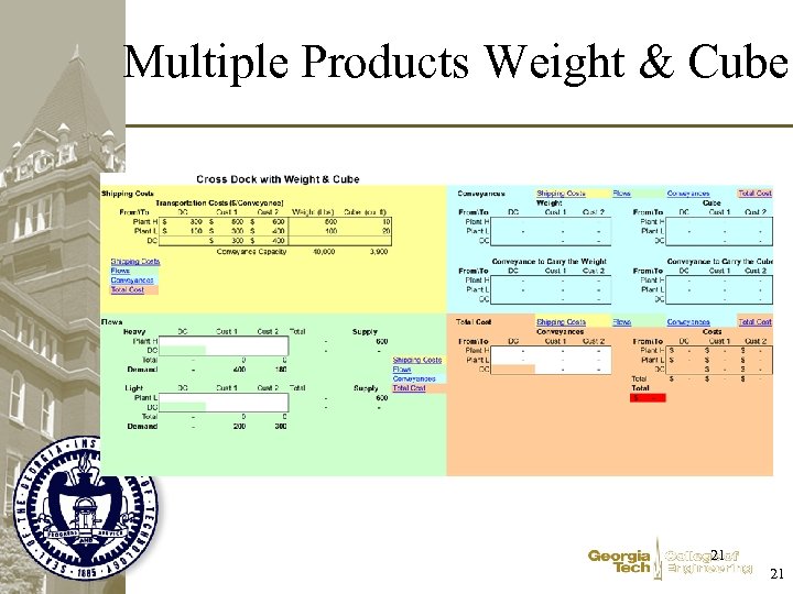
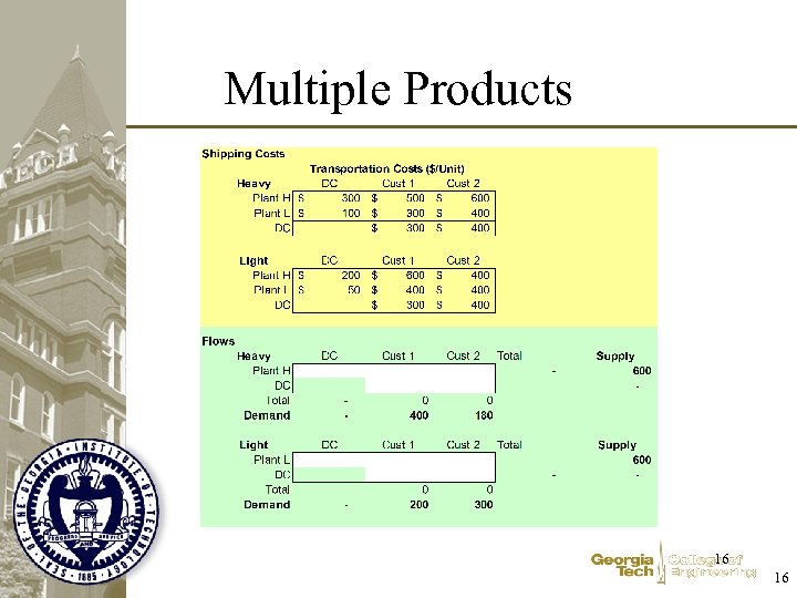Multiple Products 16 16

Conveyance Capacity • Weight Limits, e. g. , 40, 000 lbs • Cubic Capacity (53’ trailer) – 3, 970 cubic ft. – Length 52' 6" – Width 99" – Height 110" • Linear Cube (53’ trailer) – If load is not stackable, just floor space 17 17

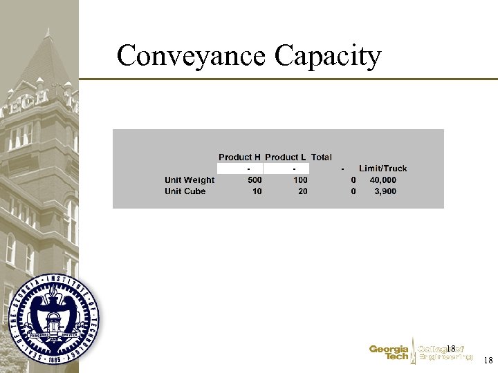Conveyance Capacity 18 18

Multiple Products Weight & Cube 19 19

Note • No Longer a Network Model • Solutions not integral • Adding integrality constraints 20 20

Multiple Products Weight & Cube 21 21

Concave Cost per unit decreasing Without special constraints, what will solver do? Shipment Size 22 22

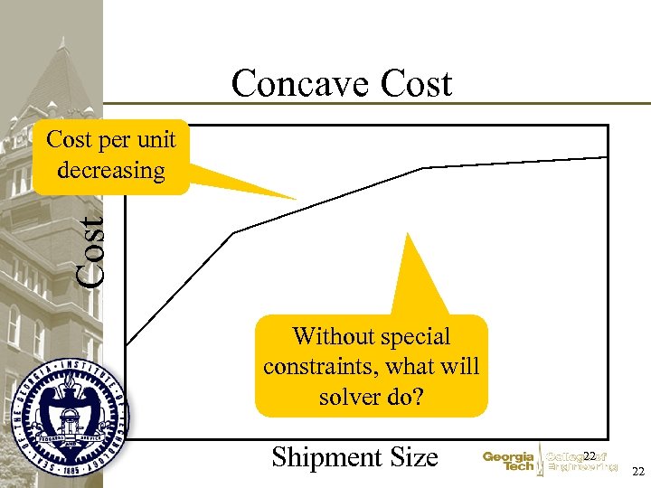
Modeling Economies of Scale • Linear Programming – Greedy – Takes the High-Range Unit Cost first! • Integer Programming – Add constraints to ensure first things first – Several Strategies 23 23

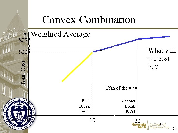Convex Combination • Weighted Average $27 What will the cost be? Total Cost $22 1/5 th of the way First Break Point 0 10 Second Break Point Mid Point 20 24 24

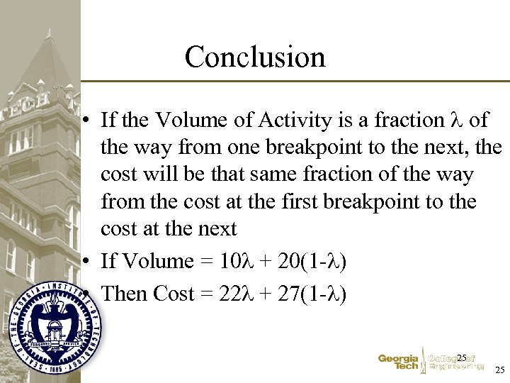Conclusion • If the Volume of Activity is a fraction of the way from one breakpoint to the next, the cost will be that same fraction of the way from the cost at the first breakpoint to the cost at the next • If Volume = 10 + 20(1 - ) • Then Cost = 22 + 27(1 - ) 25 25

Idea • Express Volume of Activity as a Weighted Average of Breakpoints • Express Cost as the same Weighted Average of Costs at the Breaks • Activity = Min Level 0 + Break 1 1 + Break 2 2 + Max Level 3 • Cost = Cost at Min Level 0 + Cost at Break 1 1 + Cost at Break 2 2 + Cost at Max Level 3 • 1 = 0 + 1 + 2 + 3 26 26

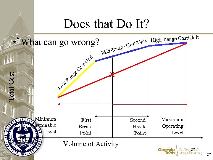Does that Do It? • What can go wrong? Total Cost U st/ o Lo Minimum Sustainable Level 0 w an R t ni e. C g nge Cost/U nit High-Ra ost/U nit e. C Rang Mid- X First Break Point Volume of Activity Second Break Point Maximum Operating Level 27 27

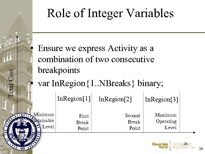Role of Integer Variables Total Cost • Ensure we express Activity as a combination of two consecutive breakpoints • var In. Region{1. . NBreaks} binary; In. Region[1] Minimum Sustainable Level First Break Point In. Region[2] Second Break Point In. Region[3] Maximum Operating Level 0 28 28

Constraints • Lambda[2] = 0 unless activity is between Total Cost – Break. Point[1] and Break. Point[2] (Region[2]) or – Break. Point[2] and Break. Point[3] (Region[3]) • Lambda[2] In. Region[2] + In. Region[3]; In. Region[1] Minimum Sustainable Level Break. Point[0] First Break Point Break. Point[1] In. Region[2] In. Region[3] Second Break Point Break. Point[2] Maximum Operating Level Break. Point[3] 29 29

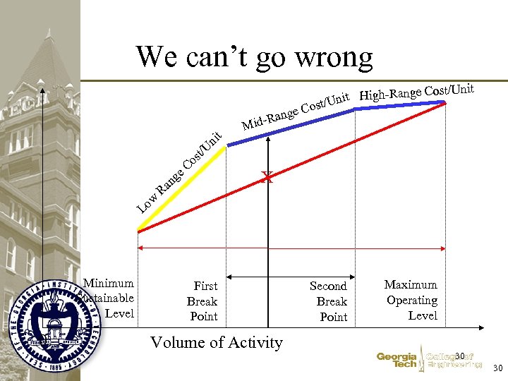We can’t go wrong nge Cost/U nit High-Ra ost/U U st/ o Lo Minimum Sustainable Level 0 w an R t ni e. C g nit e. C Rang Mid- X First Break Point Volume of Activity Second Break Point Maximum Operating Level 30 30

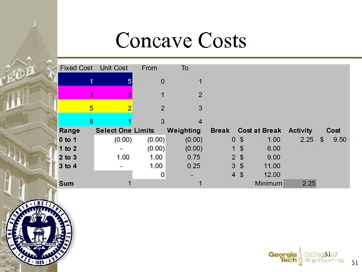Concave Costs 31 31

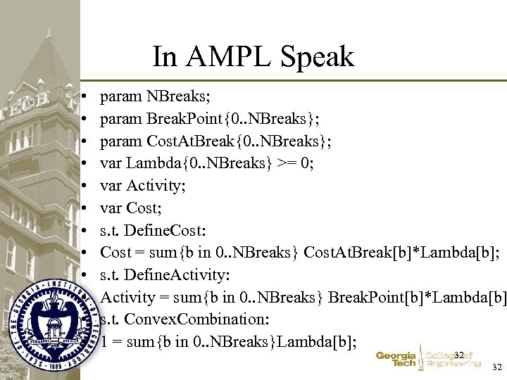In AMPL Speak • • • param NBreaks; param Break. Point{0. . NBreaks}; param Cost. At. Break{0. . NBreaks}; var Lambda{0. . NBreaks} >= 0; var Activity; var Cost; s. t. Define. Cost: Cost = sum{b in 0. . NBreaks} Cost. At. Break[b]*Lambda[b]; s. t. Define. Activity: Activity = sum{b in 0. . NBreaks} Break. Point[b]*Lambda[b] s. t. Convex. Combination: 1 = sum{b in 0. . NBreaks}Lambda[b]; 32 32

And Activity in One Region • In. Region[1] + In. Region[2] + In. Region[3] 1 • Why 1? • If it is in Region[2]: – Lambda[1] In. Region[1] + In. Region[2] = 1 – Lambda[2] In. Region[2] + In. Region[3] = 1 – Other Lambda’s are 0 33 33

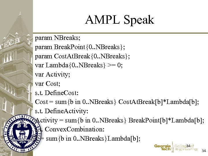AMPL Speak param NBreaks; param Break. Point{0. . NBreaks}; param Cost. At. Break{0. . NBreaks}; var Lambda{0. . NBreaks} >= 0; var Activity; var Cost; s. t. Define. Cost: Cost = sum{b in 0. . NBreaks} Cost. At. Break[b]*Lambda[b]; s. t. Define. Activity: Activity = sum{b in 0. . NBreaks} Break. Point[b]*Lambda[b]; s. t. Convex. Combination: 1 = sum{b in 0. . NBreaks}Lambda[b]; 34 34

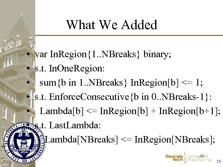What We Added • • • var In. Region{1. . NBreaks} binary; s. t. In. One. Region: sum{b in 1. . NBreaks} In. Region[b] <= 1; s. t. Enforce. Consecutive{b in 0. . NBreaks-1}: Lambda[b] <= In. Region[b] + In. Region[b+1]; s. t. Last. Lambda: – Lambda[NBreaks] <= In. Region[NBreaks]; 35 35

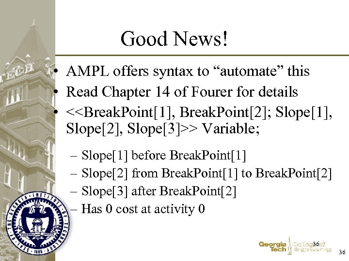Good News! • AMPL offers syntax to “automate” this • Read Chapter 14 of Fourer for details • <> Variable; – Slope[1] before Break. Point[1] – Slope[2] from Break. Point[1] to Break. Point[2] – Slope[3] after Break. Point[2] – Has 0 cost at activity 0 36 36

Modeling Time • Incorporating Schedules into Network Flow Models • Example – Given several scheduled pick-ups and deliveries (must pick-up and deliver ontime) – Question: How many vehicles required? – Assumption: One load on a vehicle at a time (No shared capacity) 37 37

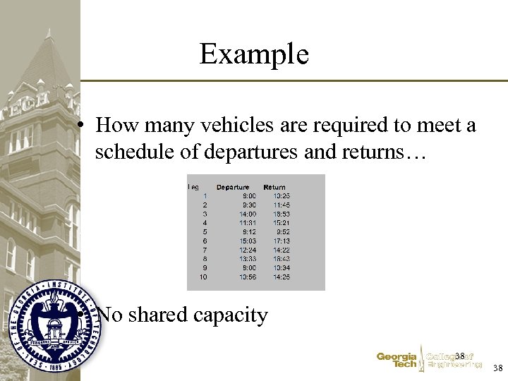Example • How many vehicles are required to meet a schedule of departures and returns… • No shared capacity 38 38

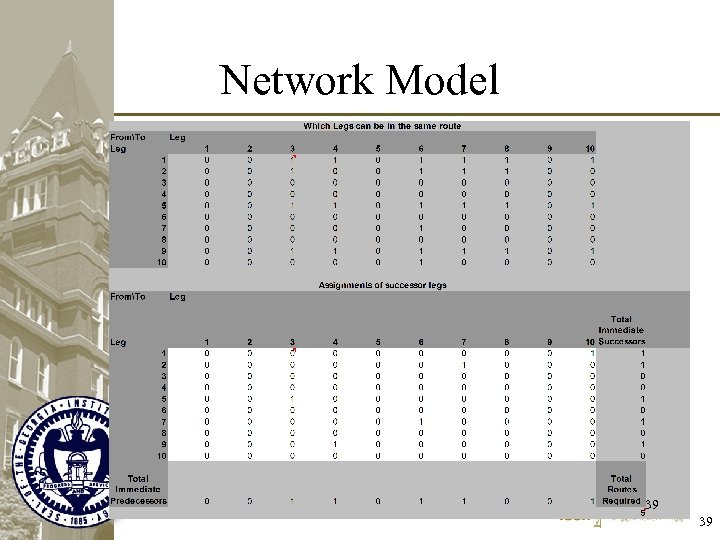Network Model 39 39

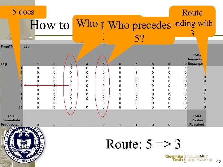5 does How to Route Who precedes ending Construct the Routes? with 3 3? 5? Route: 5 => 3 40 40

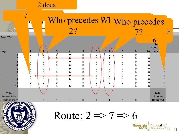2 does 7 does Who precedes the Routes? How to Construct. Who precedes Route 2? 6? 7? ending with 6 Route: 2 => 7 => 6 41 41

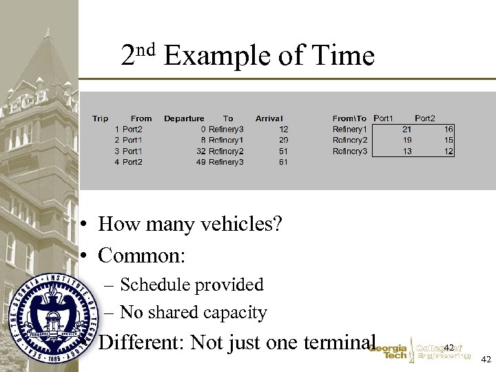2 nd Example of Time • How many vehicles? • Common: – Schedule provided – No shared capacity • Different: Not just one terminal 42 42

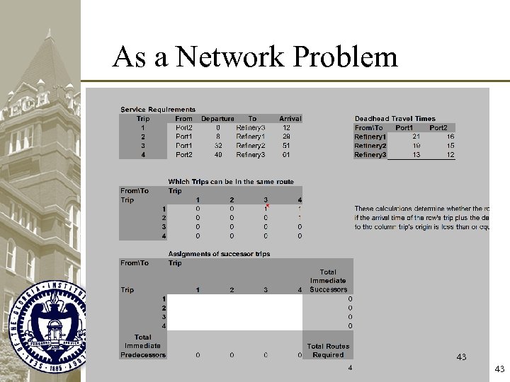As a Network Problem 43 43

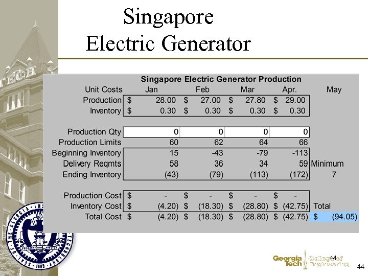Singapore Electric Generator 44 44

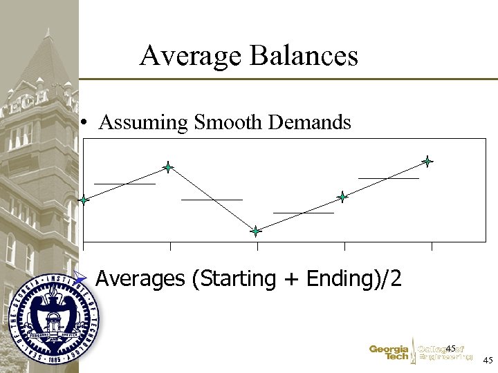Average Balances • Assuming Smooth Demands Ø Averages (Starting + Ending)/2 45 45

Inventory • Balancing Your Checkbook – Previous Balance + Income - Expenses = New Balance • Modeling Dynamic Inventory – Starting Inv. + Production - Shipments = Ending Inv. 46 46

Singapore Electric Generator 47 47

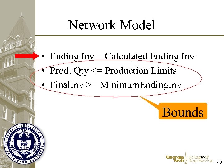Network Model • Ending Inv = Calculated Ending Inv • Prod. Qty <= Production Limits • Final. Inv >= Minimum. Ending. Inv Bounds 48 48

Network Model • Ending Inv = Calculated Ending Inv • How Many constraints is this? • Which constraints does Ending Inv for Jan appear in? • With what coefficients? • Which constraints does Production Qty in February appear in? 49 49

Summary • Network Flows – Transportation • Supply & Demand – Minimum Cost Flows • Supply, Demand &Flow conservation • Multicommodity Flows – Conserve flow of each commodity • Weight, Cube & Conveyances – Not a network flow model – Non-integral solutions • Non-Linear Costs – Requires integer variables • Modeling Time 50 50

Next • Inventory – Deterministic (predominantly) • Pipeline • Cycle – Stochastic (later) • Safety stock safety 51 51