Model Checking CTL model checking algorithms Many slides

Model Checking CTL model checking algorithms Many slides from Tevfik Bultan

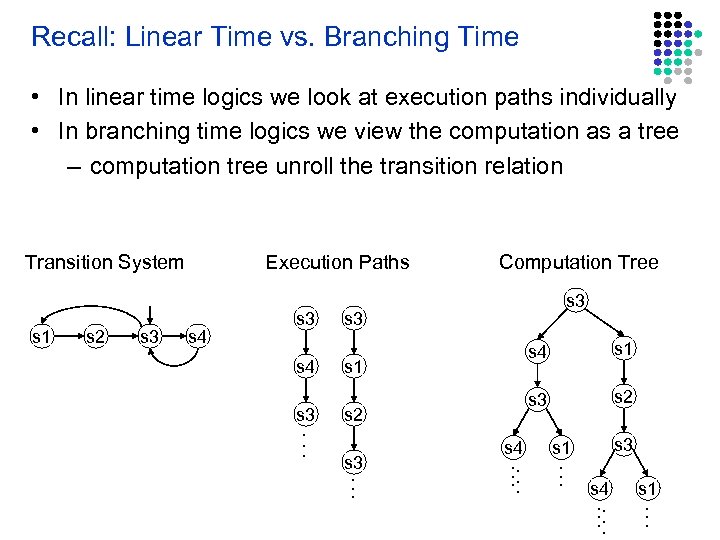Recall: Linear Time vs. Branching Time • In linear time logics we look at execution paths individually • In branching time logics we view the computation as a tree – computation tree unroll the transition relation Transition System s 1 s 2 s 3 Execution Paths s 4 s 3. . . Computation Tree s 3 s 4 s 3 s 1 s 2 s 3. . . s 4. . . s 1 s 2 s 3 s 1. . . s 4. . . s 1. . .

Recall: Computation Tree Logic (CTL) • In CTL we quantify over the paths in the computation tree • We use the same temporal operators as in LTL: X, G, F, U • We attach path quantifiers to these temporal operators: – A : for all paths – E : there exists a path • We end up with eight temporal operators: – AX, EX, AG, EG, AF, EF, AU, EU

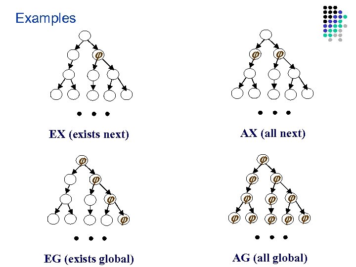Examples EX (exists next) AX (all next) EG (exists global) AG (all global)

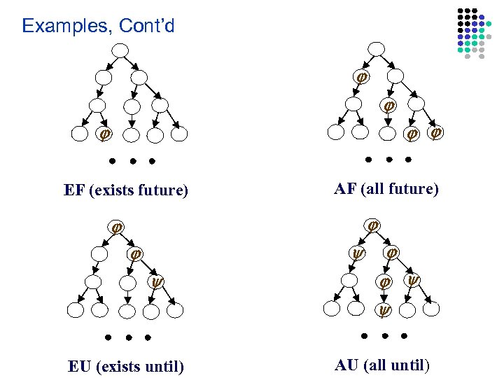Examples, Cont’d EF (exists future) AF (all future) EU (exists until) AU (all until)

Automated Verification of Finite State Systems [Clarke and Emerson 81], [Queille and Sifakis 82] • CTL Model checking problem: Given a transition system T = (S, I, R), and a CTL formula f, does the transition system satisfy the property? CTL model checking problem can be solved in O(|f| (|S|+|R|)) Note that the complexity is linear in the size of the transition system – But, the size of the transition system is exponential in the number of variables and concurrent components – this is called the state space explosion problem

CTL Model Checking Algorithm • Translate the formula to a formula which uses the basis – EX p, EG p, p EU q • Key idea: Start from the innermost (non-atomic) subformulas and label the states in the transition system with the subformulas that hold in that state – Initially states are labeled with atomic properties • Each (temporal or boolean) operator has to be processed once – Graph traversal algorithms are used to find the labeling for each operator • Computation of each subformula takes O(|S|+|R|)

CTL Model Checking Algorithm • EX p is easy to do in O(|S|+|R|) – All the nodes which have a next state labeled with p should be labeled with EX p • p EU q: Find the states which are the source of a path where p U q holds – Equivalently, find the nodes which reach a node that is labeled with q by a path where each node is labeled with p – Label such nodes with p EU q – It is a reachability problem which can be solved in O(|S|+|R|)

CTL Model Checking Algorithm • EG p: Find paths where each node is labeled with p and label nodes in such paths with EG p – First remove all the states which do not satisfy p from the transition graph – Compute the strongly connected components of the remaining graph and then find the nodes which can reach the strongly connected components (both of which can be done in O(|S|+|R|) – Label the nodes in the strongly connected components and that can reach the strongly connected components with EG p

Verification vs. Falsification • Verification: – Show: initial states truth set of p • Falsification: – Find: a state initial states truth set of p – Generate a counter-example starting from that state • CTL model checking algorithm can also generate a counterexample path if the property is not satisfied – without increasing the complexity • The ability to find counter-examples is one of the biggest strengths of the model checkers

Problems with the previous algorithm It is named to explicit state model checking • All the states and labels associated to the states must be recorded – needs a lot of memory – exponential explosion - the set of states in the transition graph is exponential to the number of variables and concurrent processes in the initial system

Temporal Properties Fixpoints [Emerson and Clarke 80] Here are some interesting CTL equivalences: AG p = p AX AG p EG p = p EX EG p AF p = p AX AF p EF p = p EX EF p p AU q = q (p AX (p AU q)) p EU q = q (p EX (p EU q)) Note that we wrote the CTL temporal operators in terms of themselves and EX and AX operators - unfolding the property

Functionals • Given a transition system T=(S, I, R), we will define functions from sets of states to sets of states – F : 2 S 2 S • For example, one such function is the EX operator (which computes the precondition of a set of states) – EX : 2 S which can be defined as: EX(p) = { s | (s, s’) R and s’ p } Abuse of notation: we use p to denote the set of states which satisfy the property p , i. e. , the truth set of p.

Functionals • Now, we can think of all temporal operators also as functions from sets of states to sets of states • For example: AX p = EX( p) or if we use the set notation AX p = (S - EX(S - p)) Abuse of notation: we will use the set and logic notations interchangeably. Logic p q p False True Set p q S–p S

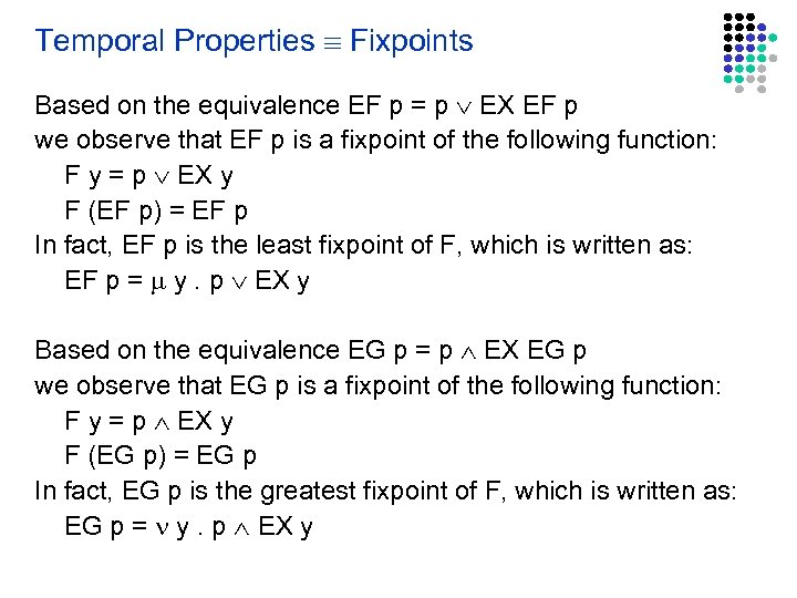Temporal Properties Fixpoints Based on the equivalence EF p = p EX EF p we observe that EF p is a fixpoint of the following function: F y = p EX y F (EF p) = EF p In fact, EF p is the least fixpoint of F, which is written as: EF p = y. p EX y Based on the equivalence EG p = p EX EG p we observe that EG p is a fixpoint of the following function: F y = p EX y F (EG p) = EG p In fact, EG p is the greatest fixpoint of F, which is written as: EG p = y. p EX y

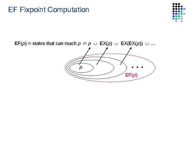EF Fixpoint Computation EF(p) states that can reach p p p EX(p) EX(EX(p)) . . . • • • EF(p)

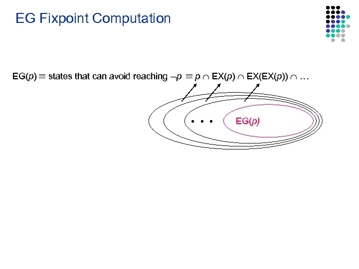EG Fixpoint Computation EG(p) states that can avoid reaching p p EX(p) EX(EX(p)) . . . • • • EG(p)

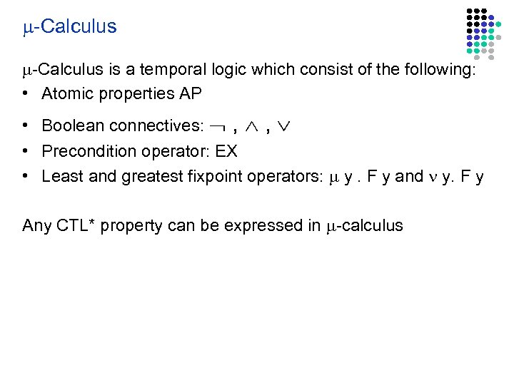-Calculus is a temporal logic which consist of the following: • Atomic properties AP • Boolean connectives: , , • Precondition operator: EX • Least and greatest fixpoint operators: y. F y and y. F y Any CTL* property can be expressed in -calculus

Symbolic Model Checking [Mc. Millan et al. LICS 90] • Represent sets of states and the transition relation as Boolean logic formulas • Fixpoint computation becomes formula manipulation – pre-condition (EX) computation: Existential variable elimination – conjunction (intersection), disjunction (union) and negation (set difference), and equivalence check • Use an efficient data structure for boolean logic formulas – Binary Decision Diagrams (BDDs)

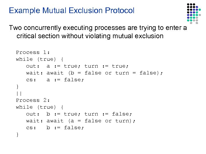Example Mutual Exclusion Protocol Two concurrently executing processes are trying to enter a critical section without violating mutual exclusion Process 1: while (true) { out: a : = true; turn : = true; wait: await (b = false or turn = false); cs: a : = false; } || Process 2: while (true) { out: b : = true; turn : = false; wait: await (a = false or turn); cs: b : = false; }

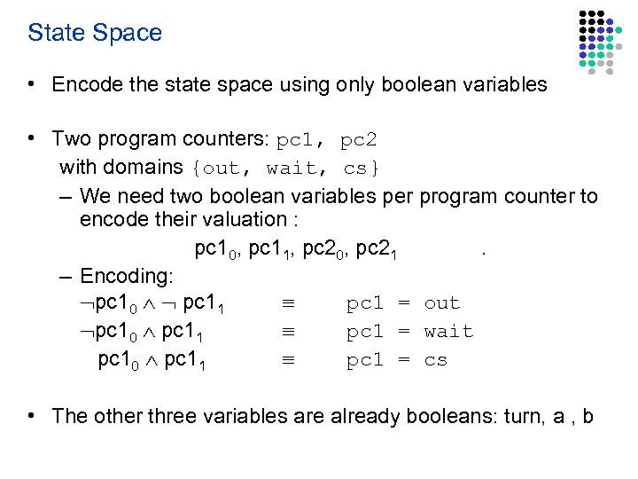State Space • Encode the state space using only boolean variables • Two program counters: pc 1, pc 2 with domains {out, wait, cs} – We need two boolean variables per program counter to encode their valuation : pc 10, pc 11, pc 20, pc 21. – Encoding: pc 10 pc 11 pc 1 = out pc 10 pc 11 pc 1 = wait pc 10 pc 11 pc 1 = cs • The other three variables are already booleans: turn, a , b

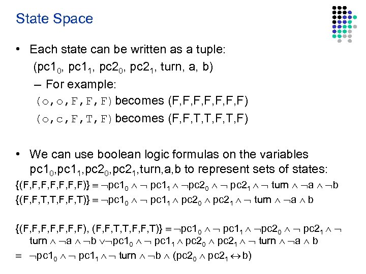State Space • Each state can be written as a tuple: (pc 10, pc 11, pc 20, pc 21, turn, a, b) – For example: (o, o, F, F, F)becomes (F, F, F, F) (o, c, F, T, F)becomes (F, F, T, T, F) • We can use boolean logic formulas on the variables pc 10, pc 11, pc 20, pc 21, turn, a, b to represent sets of states: {(F, F, F, F)} pc 10 pc 11 pc 20 pc 21 turn a b {(F, F, T, T, F, F, T)} pc 10 pc 11 pc 20 pc 21 turn a b {(F, F, F, F), (F, F, T, T, F, F, T)} pc 10 pc 11 pc 20 pc 21 turn a b pc 10 pc 11 pc 20 pc 21 turn a b pc 10 pc 11 turn b (pc 20 pc 21 b)

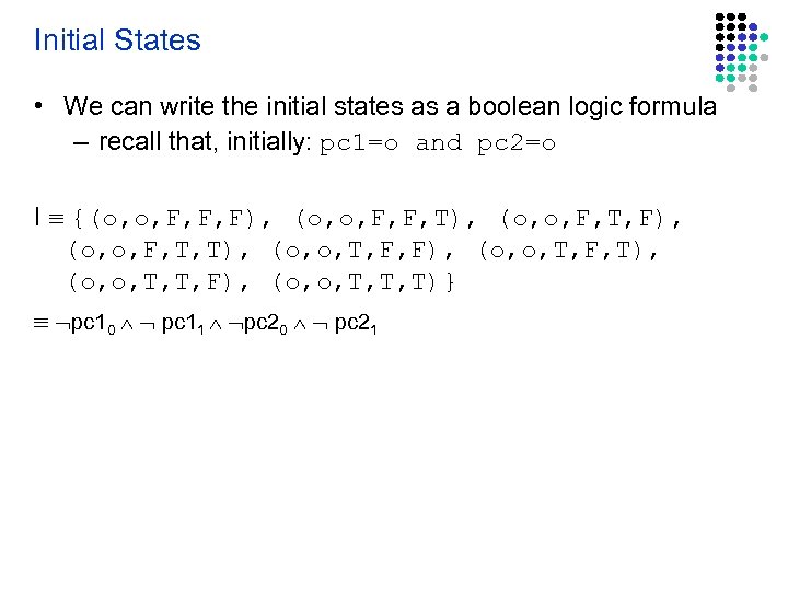Initial States • We can write the initial states as a boolean logic formula – recall that, initially: pc 1=o and pc 2=o I {(o, o, F, F, F), (o, o, F, F, T), (o, o, F, T, F), (o, o, F, T, T), (o, o, T, F, F), (o, o, T, F, T), (o, o, T, T, F), (o, o, T, T, T)} pc 10 pc 11 pc 20 pc 21

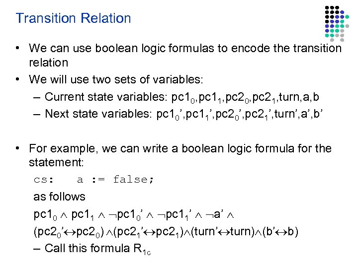Transition Relation • We can use boolean logic formulas to encode the transition relation • We will use two sets of variables: – Current state variables: pc 10, pc 11, pc 20, pc 21, turn, a, b – Next state variables: pc 10’, pc 11’, pc 20’, pc 21’, turn’, a’, b’ • For example, we can write a boolean logic formula for the statement: cs: a : = false; as follows pc 10 pc 11 pc 10’ pc 11’ a’ (pc 20’ pc 20) (pc 21’ pc 21) (turn’ turn) (b’ b) – Call this formula R 1 c

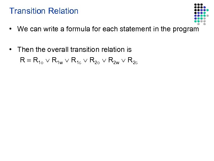Transition Relation • We can write a formula for each statement in the program • Then the overall transition relation is R R 1 o R 1 w R 1 c R 2 o R 2 w R 2 c

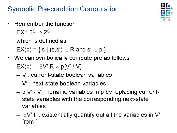Symbolic Pre-condition Computation • Remember the function EX : 2 S which is defined as: EX(p) = { s | (s, s’) R and s’ p } • We can symbolically compute pre as follows EX(p) V’ R p[V’ / V] – V : current-state boolean variables – V’ : next-state boolean variables – p[V’ / V] : rename variables in p by replacing currentstate variables with the corresponding next-state variables – V’ f : existentially quantify out all the variables in V’ from f

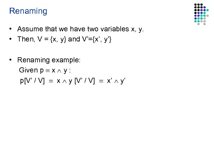Renaming • Assume that we have two variables x, y. • Then, V = {x, y} and V’={x’, y’} • Renaming example: Given p x y : p[V’ / V] x y [V’ / V] x’ y’

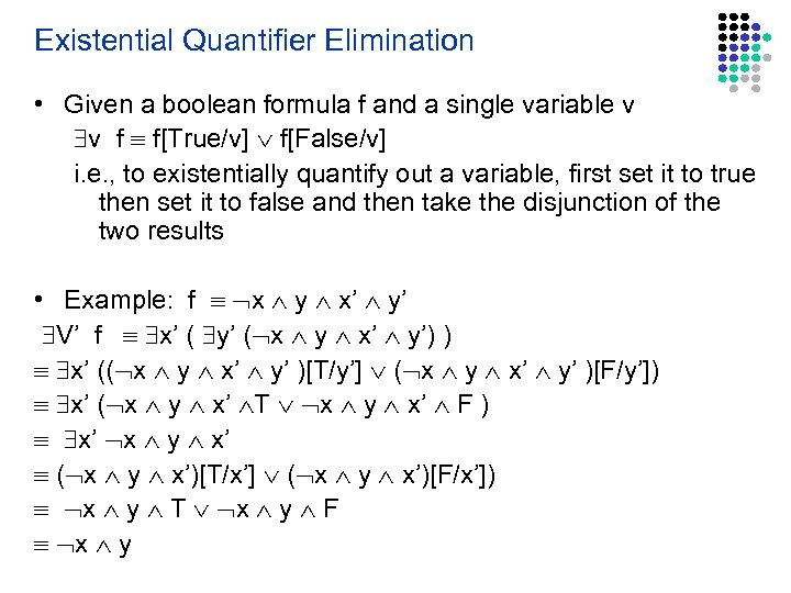Existential Quantifier Elimination • Given a boolean formula f and a single variable v v f f[True/v] f[False/v] i. e. , to existentially quantify out a variable, first set it to true then set it to false and then take the disjunction of the two results • Example: f x y x’ y’ V’ f x’ ( y’ ( x y x’ y’) ) x’ (( x y x’ y’ )[T/y’] ( x y x’ y’ )[F/y’]) x’ ( x y x’ T x y x’ F ) x’ x y x’ ( x y x’)[T/x’] ( x y x’)[F/x’]) x y T x y F x y

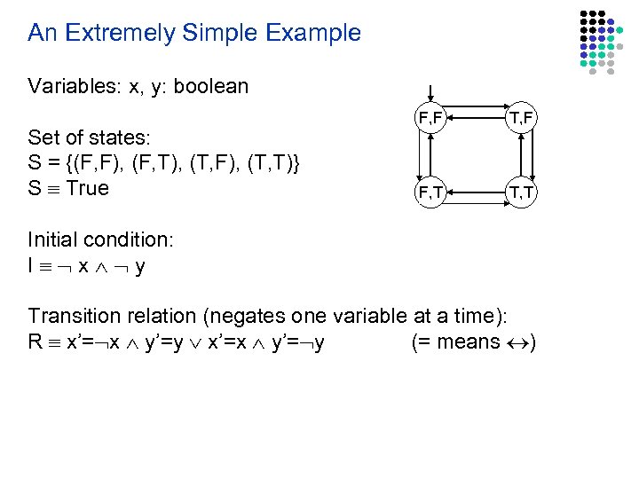An Extremely Simple Example Variables: x, y: boolean Set of states: S = {(F, F), (F, T), (T, F), (T, T)} S True F, F T, F F, T T, T Initial condition: I x y Transition relation (negates one variable at a time): R x’= x y’=y x’=x y’= y (= means )

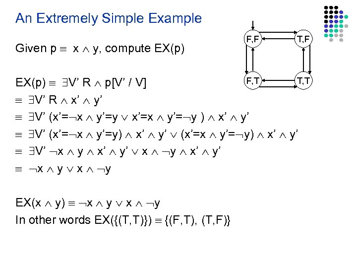An Extremely Simple Example Given p x y, compute EX(p) F, F T, F F, T T, T EX(p) V’ R p[V’ / V] V’ R x’ y’ V’ (x’= x y’=y x’=x y’= y ) x’ y’ V’ (x’= x y’=y) x’ y’ (x’=x y’= y) x’ y’ V’ x y x’ y’ x y EX(x y) x y In other words EX({(T, T)}) {(F, T), (T, F)}

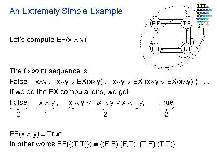An Extremely Simple Example 3 F, F T, F Let’s compute EF(x y) 2 1 F, T The fixpoint sequence is False, x y EX(x y) , x y EX (x y EX(x y) ) , . . . If we do the EX computations, we get: False, x y x y, True 0 1 2 3 EF(x y) True In other words EF({(T, T)}) {(F, F), (F, T), (T, F), (T, T)}

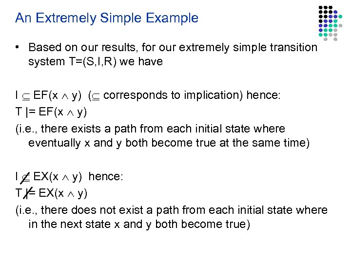An Extremely Simple Example • Based on our results, for our extremely simple transition system T=(S, I, R) we have I EF(x y) ( corresponds to implication) hence: T |= EF(x y) (i. e. , there exists a path from each initial state where eventually x and y both become true at the same time) I EX(x y) hence: T |= EX(x y) (i. e. , there does not exist a path from each initial state where in the next state x and y both become true)

An Extremely Simple Example • Let’s try one more property AF(x y) • To check this property we first convert it to a formula which uses only the temporal operators in our basis: AF(x y) EG( (x y)) If we can find an initial state which satisfies EG( (x y)), then we know that the transition system T, does not satisfy the property AF(x y)

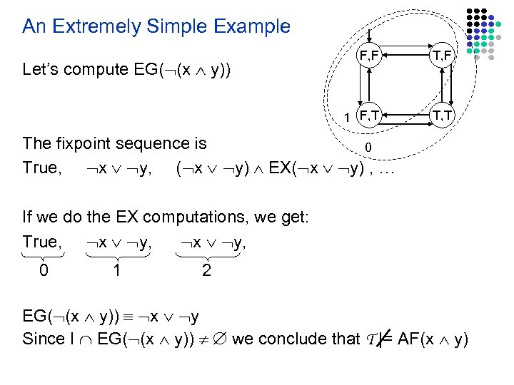An Extremely Simple Example T, F 1 F, T Let’s compute EG( (x y)) F, F T, T The fixpoint sequence is 0 True, x y, ( x y) EX( x y) , … If we do the EX computations, we get: True, x y, 0 1 2 EG( (x y)) x y Since I EG( (x y)) we conclude that T |= AF(x y)

Symbolic CTL Model Checking Algorithm • Translate the formula to a formula which uses the basis – EX p, EG p, p EU q • Atomic formulas can be interpreted directly on the state representation • For EX p compute the precondition using existential variable elimination as we discussed • For EG and EU compute the fixpoints iteratively

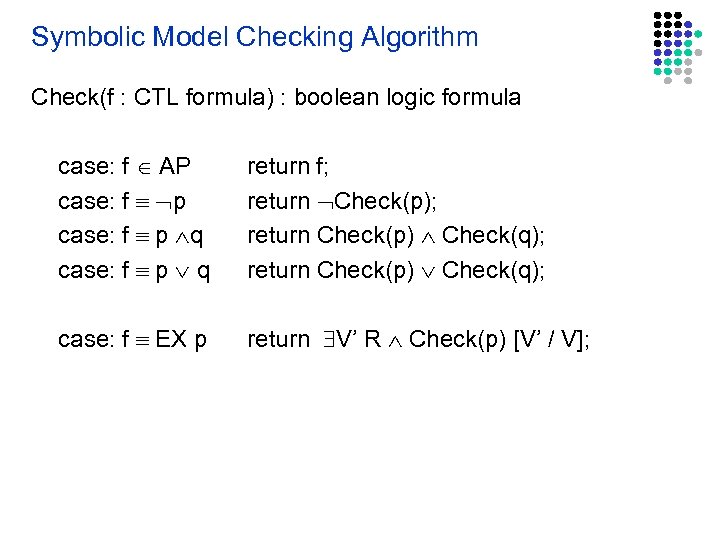Symbolic Model Checking Algorithm Check(f : CTL formula) : boolean logic formula case: f AP case: f p q case: f p q return f; return Check(p) Check(q); case: f EX p return V’ R Check(p) [V’ / V];

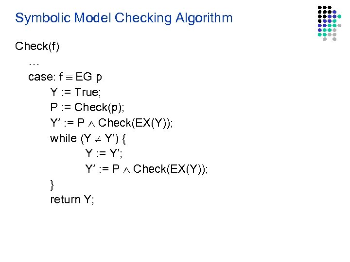Symbolic Model Checking Algorithm Check(f) … case: f EG p Y : = True; P : = Check(p); Y’ : = P Check(EX(Y)); while (Y Y’) { Y : = Y’; Y’ : = P Check(EX(Y)); } return Y;

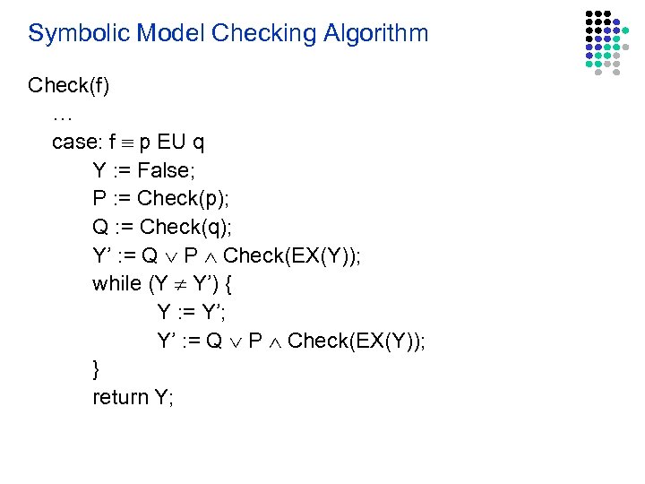Symbolic Model Checking Algorithm Check(f) … case: f p EU q Y : = False; P : = Check(p); Q : = Check(q); Y’ : = Q P Check(EX(Y)); while (Y Y’) { Y : = Y’; Y’ : = Q P Check(EX(Y)); } return Y;

Binary Decision Diagrams (BDDs) • Ordered Binary Decision Diagrams (BDDs) – An efficient data structure for boolean formula manipulation – There are BDD packages available: (for example CUDD from Colorado University) • BDD data structure can be used to implement the symbolic model checking algorithm discussed above • BDDs are a canonical representation for boolean logic formulas – given two boolean logic formulas F and G, if F and G are equivalent their BDD representations will be identical

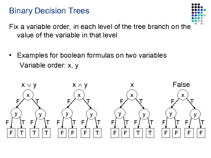Binary Decision Trees Fix a variable order, in each level of the tree branch on the value of the variable in that level • Examples for boolean formulas on two variables Variable order: x, y x y x False x x F T y F F y y T F F T T T F F y y T F F T F T F F F y y T F T T T F F y T F F F

BDDs • Repeatedly apply the following transformations to a binary decision tree: – Remove duplicate terminals – Remove duplicate non-terminals – Remove redundant tests • These transformations transform the tree to a directed acyclic graph

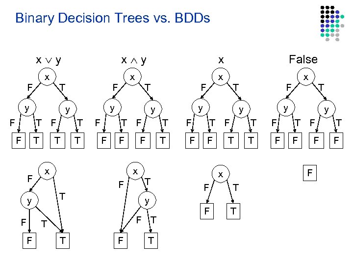Binary Decision Trees vs. BDDs x y x False x x F T y F F y y T F F T F F T T y T F x T F y x y T F F F y y T F T T F F y T F F F F x F T T

Good News About BDDs • Given BDDs for two boolean logic formulas F and G – The BDDs for F G and F G are of size |F| |G| (and can be computed in that time) – The BDD for F is of size |F| (and can be computed in that time) – F ? G can be checked in constant time – Satisfiability of F can be checked in constant time • But, this does not mean that you cane solve SAT in constant time

Bad News About BDDs • The size of a BDD can be exponential in the number of boolean variables • The sizes of the BDDs are very sensitive to the variable ordering. Bad variable ordering can cause exponential increase in the size of the BDD • There are functions which have BDDs that are exponential for any variable ordering (for example binary multiplication) • Pre condition computation requires existential variable elimination – Existential variable elimination cause an exponential blow-up in the size of the BDD

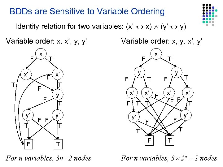BDDs are Sensitive to Variable Ordering Identity relation for two variables: (x’ x) (y' y) Variable order: x, x’, y, y' F x x’ T F T T F F F x’ T F y’ Variable order: x, y, x’, y' y T y’ T T For n variables, 3 n+2 nodes y F T T y F T x’ x’ F F T T y’ y’ F F T T For n variables, 3 2 n – 1 nodes

What About LTL and CTL* Model Checking? • The complexity of the model checking problem for LTL and CTL* are: – (|S|+|R|) 2 O(|f|) where |f| is the number of logic connectives in f • Typically the size of the formula is much smaller than the size of the transition system – So the exponential complexity in the size of the formula is not very significant in practice • LTL properties are more intuitive and easier to write correctly – XF p and FX p are equivalent in LTL – AXAF p and AFAX p are not equivalent in LTL