Model Checking Abstractions and Reductions Orna Grumberg Computer

Model Checking, Abstractions and Reductions Orna Grumberg Computer Science Department Technion Haifa, Israel 1

Overview • Temporal logic model checking • The state explosion problem • Reducing the model of the system by abstractions 2

Program verification Given a program and a specification, does the program satisfy the specification? Not decidable! We restrict the problem to a decidable one: • Finite-state reactive systems • Propositional temporal logics 3

Model Checking An efficient procedure that receives • Description of a finite-state system (model) • Property written as a formula of propositional temporal logic It returns yes, if the system has the property It returns no + counterexample, otherwise 4

Finite state systems • hardware designs • Communication protocols • High level description of non finite state systems 5

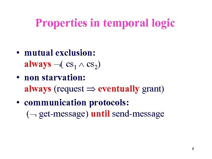
Properties in temporal logic • mutual exclusion: always ( cs 1 cs 2) • non starvation: always (request eventually grant) • communication protocols: ( get-message) until send-message 6

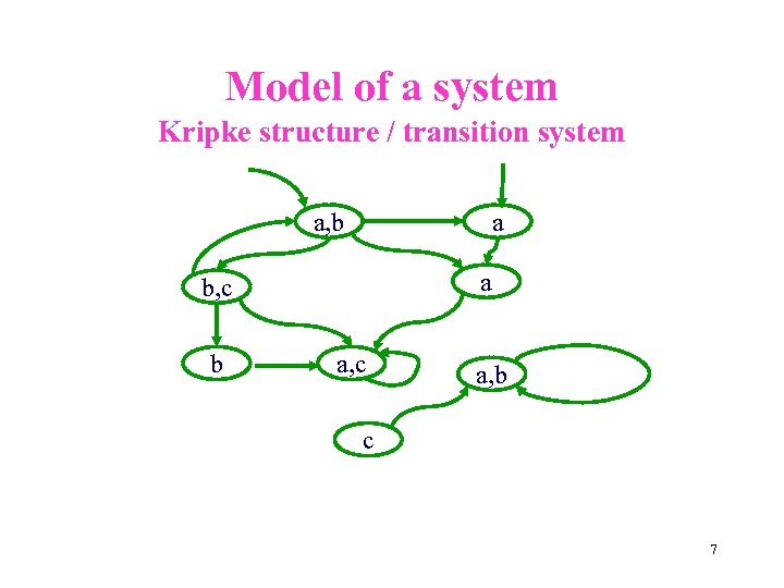
Model of a system Kripke structure / transition system a, b a a b, c b a, c a, b c 7

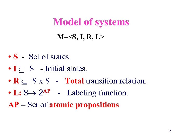
Model of systems M=<S, I, R, L> • S - Set of states. • I S - Initial states. • R S x S - Total transition relation. • L: S 2 AP - Labeling function. AP – Set of atomic propositions 8

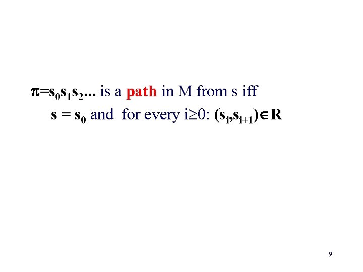
=s 0 s 1 s 2. . . is a path in M from s iff s = s 0 and for every i 0: (si, si+1) R 9

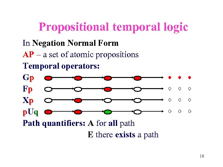
Propositional temporal logic In Negation Normal Form AP – a set of atomic propositions Temporal operators: Gp Fp Xp p. Uq Path quantifiers: A for all path E there exists a path 10

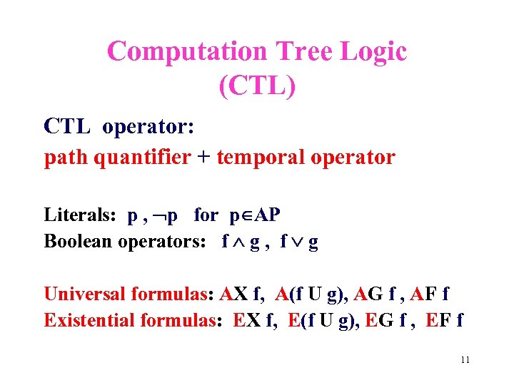
Computation Tree Logic (CTL) CTL operator: path quantifier + temporal operator Literals: p , p for p AP Boolean operators: f g , f g Universal formulas: AX f, A(f U g), AG f , AF f Existential formulas: EX f, E(f U g), EG f , EF f 11

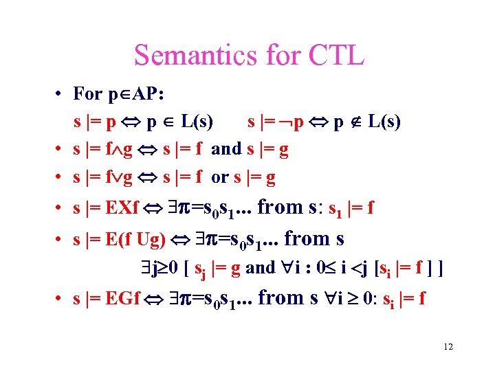
Semantics for CTL • For p AP: s |= p p L(s) • s |= f g s |= f and s |= g • s |= f g s |= f or s |= g • s |= EXf =s 0 s 1. . . from s: s 1 |= f • s |= E(f Ug) =s 0 s 1. . . from s j 0 [ sj |= g and i : 0 i j [si |= f ] ] • s |= EGf =s 0 s 1. . . from s i 0: si |= f 12

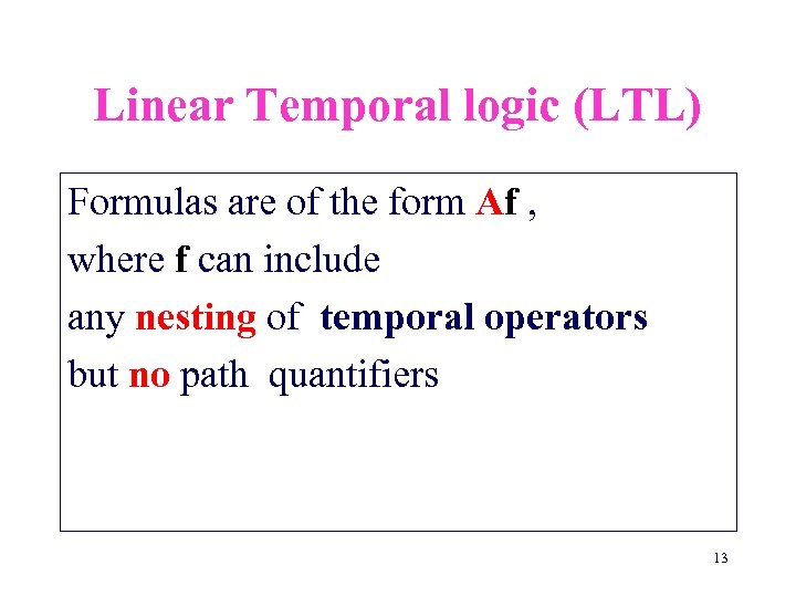
Linear Temporal logic (LTL) Formulas are of the form Af , where f can include any nesting of temporal operators but no path quantifiers 13

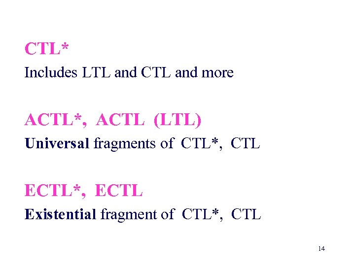
CTL* Includes LTL and CTL and more ACTL*, ACTL (LTL) Universal fragments of CTL*, CTL ECTL*, ECTL Existential fragment of CTL*, CTL 14

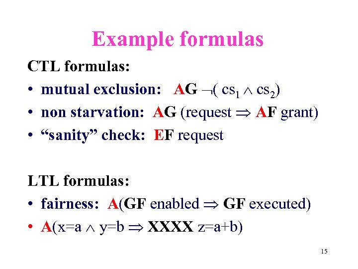
Example formulas CTL formulas: • mutual exclusion: AG ( cs 1 cs 2) • non starvation: AG (request AF grant) • “sanity” check: EF request LTL formulas: • fairness: A(GF enabled GF executed) • A(x=a y=b XXXX z=a+b) 15

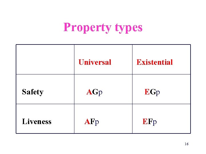
Property types Universal Existential Safety AGp EGp Liveness AFp EFp 16

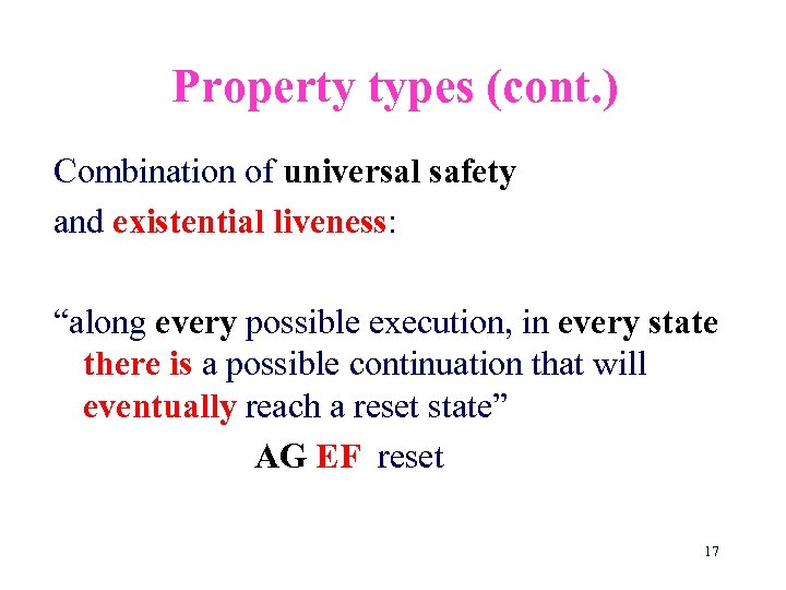
Property types (cont. ) Combination of universal safety and existential liveness: “along every possible execution, in every state there is a possible continuation that will eventually reach a reset state” AG EF reset 17

Model Checking M |= f [Clarke, Emerson, Sistla 83] • The Model Checking algorithm works iteratively on subformulas of f , from simpler subformulas to more complex ones • When checking subformula g of f we assume that all subformulas of g have already been checked • For subformula g, the algorithm returns the set of states that satisfy g ( Sg ) • The algorithm has time complexity: O( |M| |f| ) 18

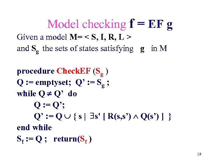
Model checking f = EF g Given a model M= < S, I, R, L > and Sg the sets of states satisfying g in M procedure Check. EF (Sg ) Q : = emptyset; Q’ : = Sg ; while Q Q’ do Q : = Q’; Q’ : = Q { s | s' [ R(s, s’) Q(s’) ] } end while Sf : = Q ; return(Sf ) 19

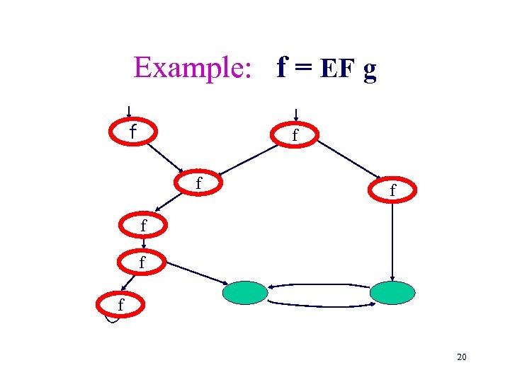
Example: f = EF g f f f g f 20

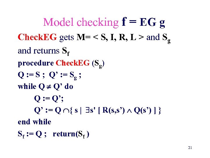
Model checking f = EG g Check. EG gets M= < S, I, R, L > and Sg and returns Sf procedure Check. EG (Sg) Q : = S ; Q’ : = Sg ; while Q Q’ do Q : = Q’; Q’ : = Q { s | s' [ R(s, s’) Q(s’) ] } end while Sf : = Q ; return(Sf ) 21

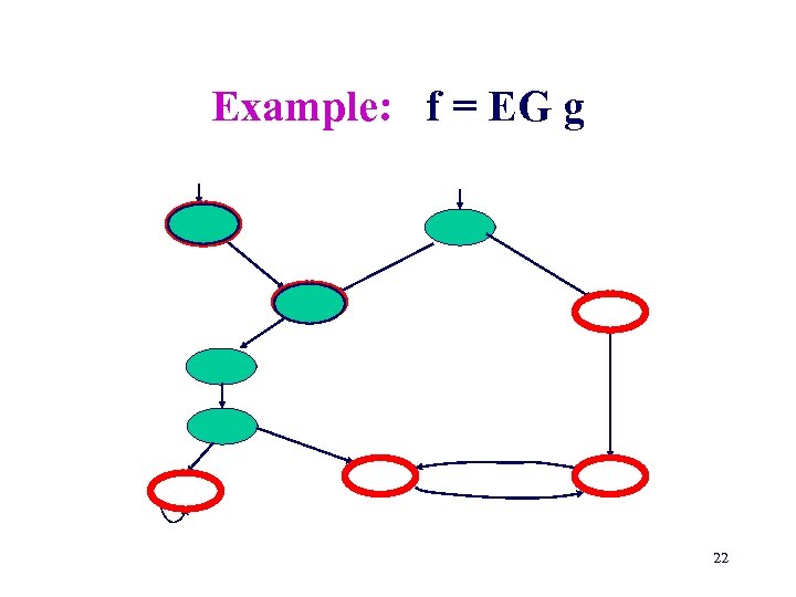
Example: f = EG g g g g 22

Symbolic model checking [Burch, Clarke, Mc. Millan, Dill 1990] If the model is given explicitly (e. g. by adjacent matrix) then only systems with about ten Boolean variables (~1000 states) can be handled Symbolic model checking uses Binary Decision Diagrams ( BDDs ) to represent the model and sets of states. It can handle systems with hundreds of Boolean variables. 23

Binary decision diagrams (BDDs) [Bryant 86] • Data structure for representing Boolean functions • Often concise in memory • Canonical representation • Boolean operations on BDDs can be done in polynomial time in the BDD size 24

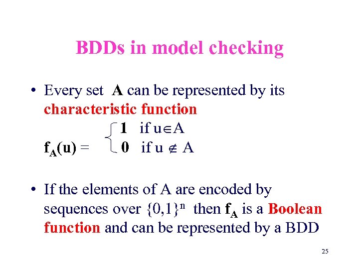
BDDs in model checking • Every set A can be represented by its characteristic function 1 if u A f. A(u) = 0 if u A • If the elements of A are encoded by sequences over {0, 1}n then f. A is a Boolean function and can be represented by a BDD 25

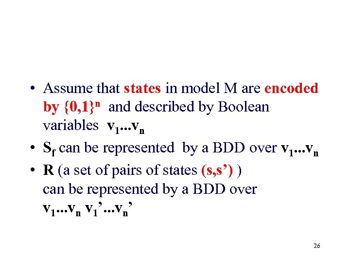
• Assume that states in model M are encoded by {0, 1}n and described by Boolean variables v 1. . . vn • Sf can be represented by a BDD over v 1. . . vn • R (a set of pairs of states (s, s’) ) can be represented by a BDD over v 1. . . vn v 1’. . . vn’ 26

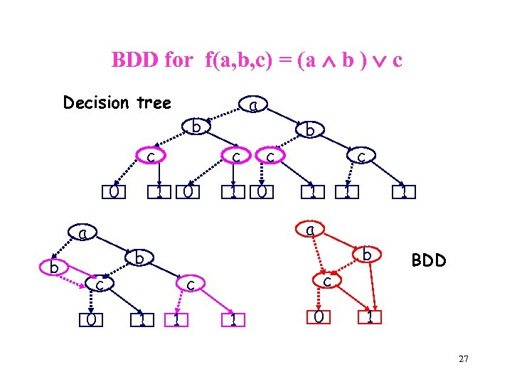
BDD for f(a, b, c) = (a b ) c Decision tree a b c 0 b c 1 0 c 1 1 1 a a b c b b c 0 c c 1 1 1 0 BDD 1 27

State explosion problem • Hardware designs are extremely large: > 106 registers • state of the art symbolic model checking can handle medium size designs effectively: a few hundreds of Boolean variables Other solutions for the state explosion problem are needed! 28

Possible solution Replacing the system model by a smaller one (less states and transitions) that still preserves properties of interest • Modular verification • Symmetry • Abstraction 29

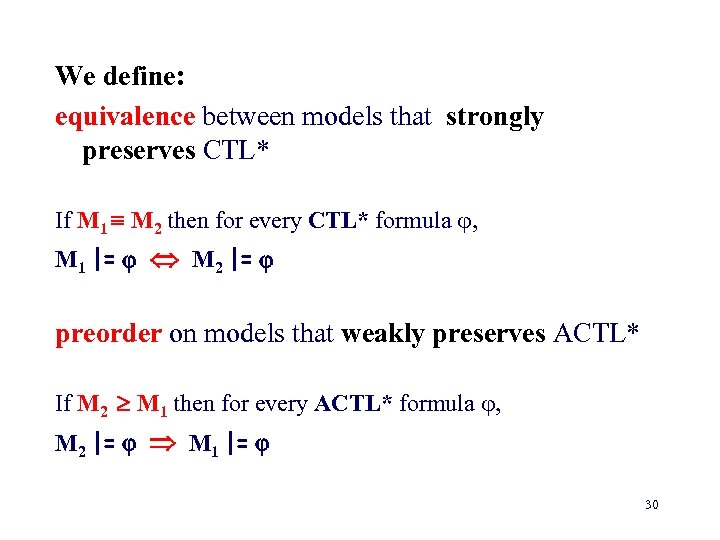
We define: equivalence between models that strongly preserves CTL* If M 1 M 2 then for every CTL* formula , M 1 |= M 2 |= preorder on models that weakly preserves ACTL* If M 2 M 1 then for every ACTL* formula , M 2 |= M 1 |= 30

The simulation preorder [Milner] Given two models M 1 = (S 1, I 1, R 1, L 1), M 2 = (S 2, I 2, R 2, L 2) H S 1 x S 2 is a simulation iff for every (s 1, s 2 ) H : • s 1 and s 2 satisfy the same propositions • For every successor t 1 of s 1 there is a successor t 2 of s 2 such that (t 1, t 2) H Notation: s 1 s 2 31

The simulation preorder [Milner] Given two models M 1 = (S 1, I 1, R 1, L 1), M 2 = (S 2, I 2, R 2, L 2) H S 1 x S 2 is a simulation iff for every (s 1, s 2 ) H : • p AP: s 2 |= p s 1 |= p • t 1 [ (s 1, t 1) R 1 t 2 [ (s 2, t 2) R 2 (t 1, t 2) H ] ] Notation: s 1 s 2 32

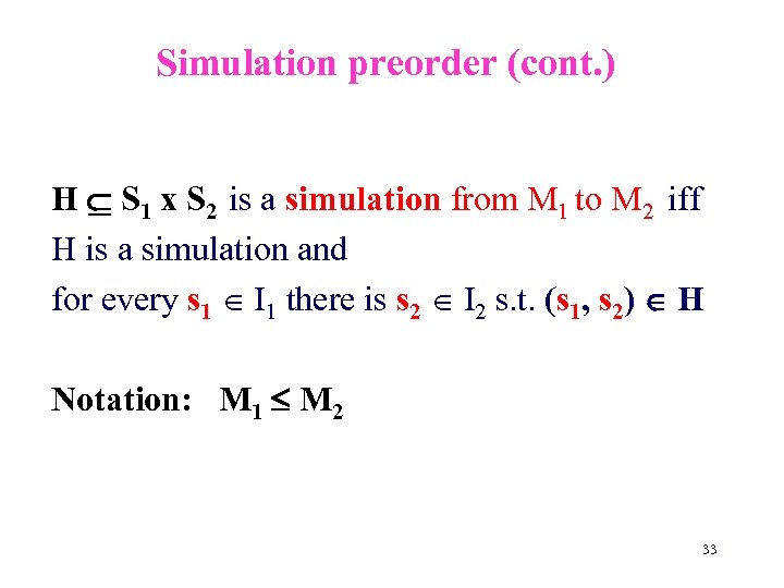
Simulation preorder (cont. ) H S 1 x S 2 is a simulation from M 1 to M 2 iff H is a simulation and for every s 1 I 1 there is s 2 I 2 s. t. (s 1, s 2) H Notation: M 1 M 2 33

Bisimulation relation [Park] For models M 1 and M 2, H S 1 x S 2 is a bisimulation iff for every (s 1, s 2 ) H : • p AP : p L(s 2) p L(s 1) • t 1 [ (s 1, t 1) R 1 t 2 [ (s 2, t 2) R 2 (t 1, t 2) H ] ] • t 2 [ (s 2, t 2) R 2 t 1 [ (s 1, t 1) R 1 (t 1, t 2) H ] ] Notation: s 1 s 2 34

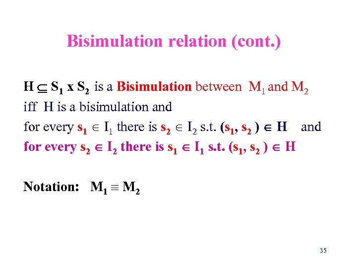
Bisimulation relation (cont. ) H S 1 x S 2 is a Bisimulation between M 1 and M 2 iff H is a bisimulation and for every s 1 I 1 there is s 2 I 2 s. t. (s 1, s 2 ) H and for every s 2 I 2 there is s 1 I 1 s. t. (s 1, s 2 ) H Notation: M 1 M 2 35

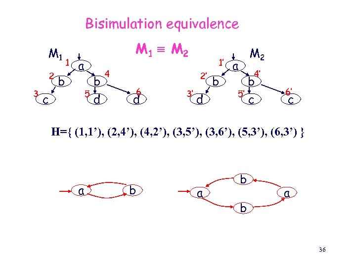
Bisimulation equivalence M 1 2 3 b 1 M 1 M 2 a 5 c b d 4 1’ 2’ 6 d 3’ d b M 2 a 4’ b 5’ c 6’ c H={ (1, 1’), (2, 4’), (4, 2’), (3, 5’), (3, 6’), (5, 3’), (6, 3’) } a b b a 36

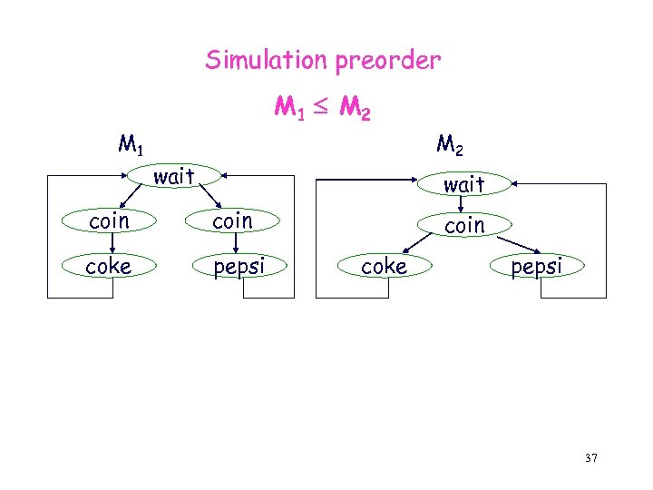
Simulation preorder M 1 M 2 M 1 M 2 wait coin coke pepsi 37

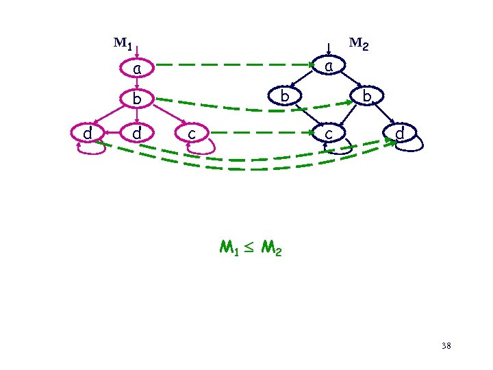
M 1 a a b b d d c M 2 b c d M 1 M 2 38

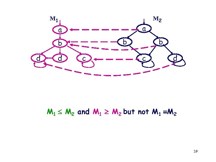
M 1 a a b b d d c M 2 b c d M 1 M 2 and M 1 M 2 but not M 1 M 2 39

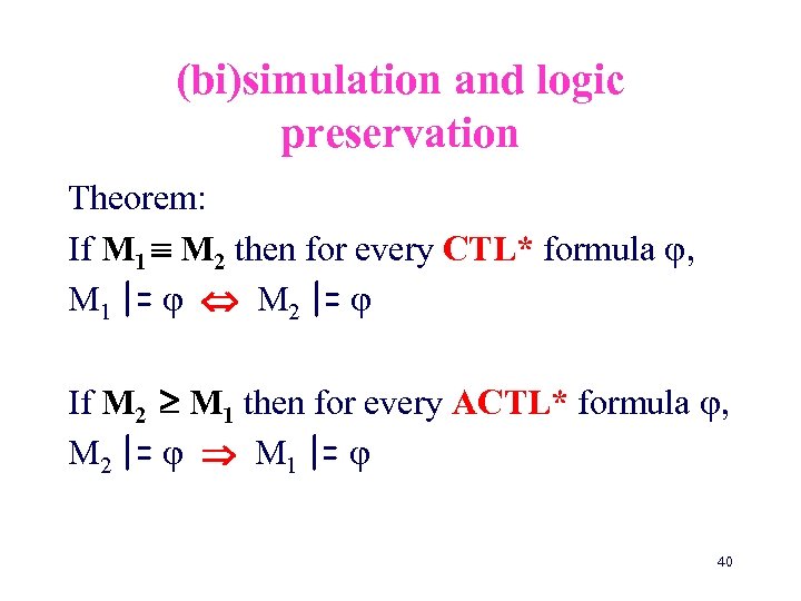
(bi)simulation and logic preservation Theorem: If M 1 M 2 then for every CTL* formula , M 1 |= M 2 |= If M 2 M 1 then for every ACTL* formula , M 2 |= M 1 |= 40

Abstractions • They are one of the most useful ways to fight the state explosion problem • They should preserve properties of interest: properties that hold for the abstract model should hold for the concrete model • Abstractions should be constructed directly from the program 41

Data abstraction Abstracts data information while still enabling to partially check properties referring to data E. Clarke, O. Grumberg, D. Long. Model checking and abstraction, TOPLAS, Vol. 16, No. 5, Sept. 1994 42

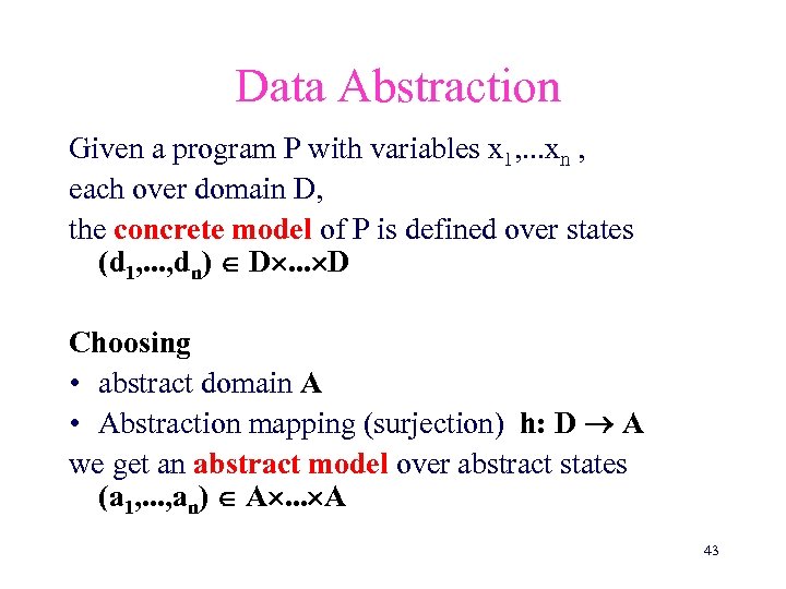
Data Abstraction Given a program P with variables x 1, . . . xn , each over domain D, the concrete model of P is defined over states (d 1, . . . , dn) D. . . D Choosing • abstract domain A • Abstraction mapping (surjection) h: D A we get an abstract model over abstract states (a 1, . . . , an) A. . . A 43

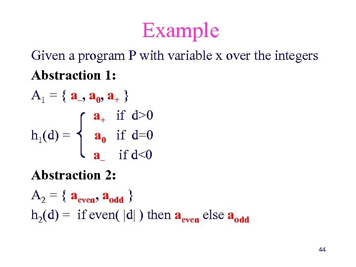
Example Given a program P with variable x over the integers Abstraction 1: A 1 = { a–, a 0, a+ } a+ if d>0 h 1(d) = a 0 if d=0 a– if d<0 Abstraction 2: A 2 = { aeven, aodd } h 2(d) = if even( |d| ) then aeven else aodd 44

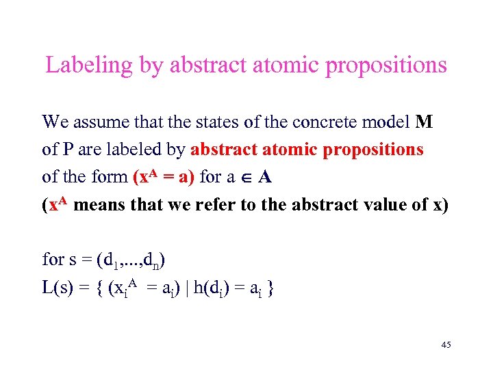
Labeling by abstract atomic propositions We assume that the states of the concrete model M of P are labeled by abstract atomic propositions of the form (x. A = a) for a A (x. A means that we refer to the abstract value of x) for s = (d 1, . . . , dn) L(s) = { (xi. A = ai) | h(di) = ai } 45

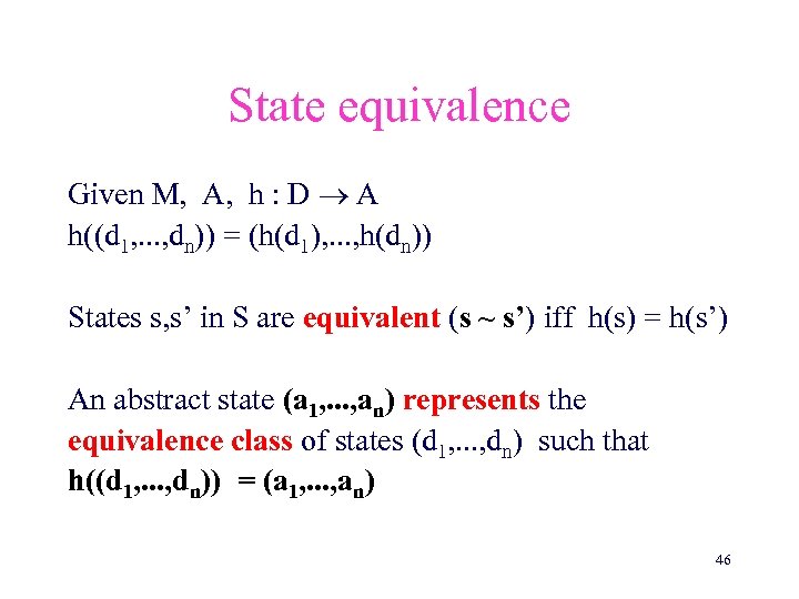
State equivalence Given M, A, h : D A h((d 1, . . . , dn)) = (h(d 1), . . . , h(dn)) States s, s’ in S are equivalent (s ~ s’) iff h(s) = h(s’) An abstract state (a 1, . . . , an) represents the equivalence class of states (d 1, . . . , dn) such that h((d 1, . . . , dn)) = (a 1, . . . , an) 46

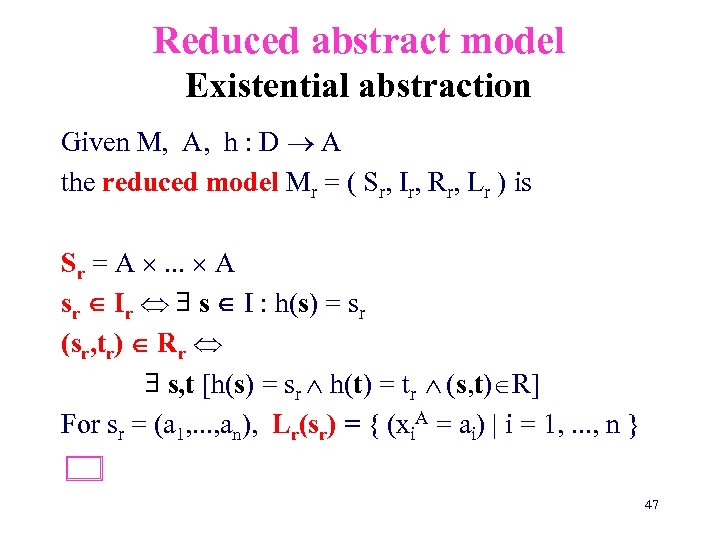
Reduced abstract model Existential abstraction Given M, A, h : D A the reduced model Mr = ( Sr, Ir, Rr, Lr ) is Sr = A . . . A sr Ir s I : h(s) = sr (sr, tr) Rr s, t [h(s) = sr h(t) = tr (s, t) R] For sr = (a 1, . . . , an), Lr(sr) = { (xi. A = ai) | i = 1, . . . , n } 47

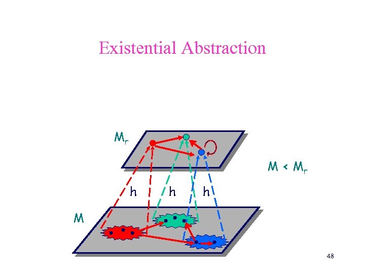
Existential Abstraction Mr M < Mr h h h M 48

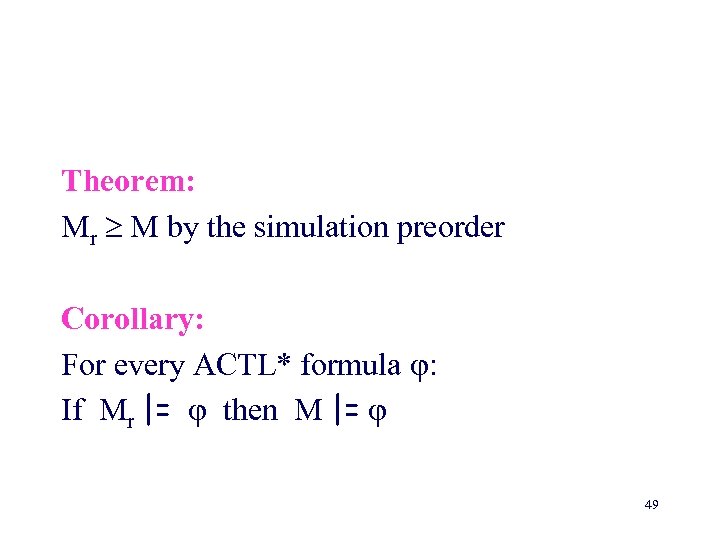
Theorem: Mr M by the simulation preorder Corollary: For every ACTL* formula : If Mr |= then M |= 49

Example Program with one variable x over the integers Initially x may be either 0 or 1 At any step, x may non-deterministically either decrease or increase by 1 50

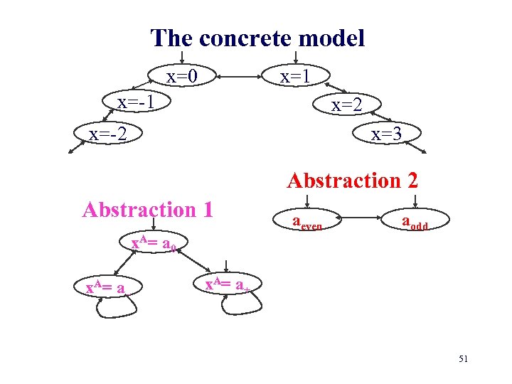
The concrete model x=0 x=1 x=-1 x=2 x=-2 x=3 Abstraction 2 Abstraction 1 aeven aodd x. A= a 0 x. A= a– x. A= a+ 51

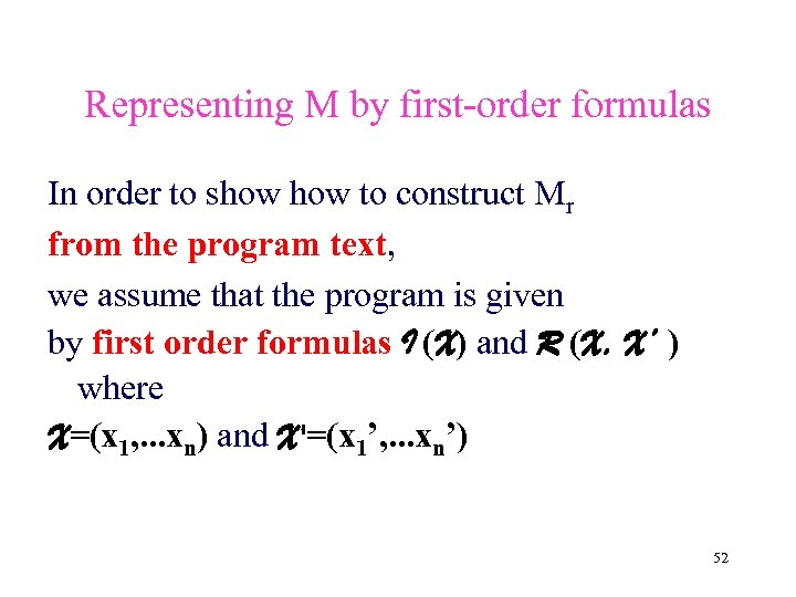
Representing M by first-order formulas In order to show to construct Mr from the program text, we assume that the program is given by first order formulas I (X) and R (X, X’ ) where X=(x 1, . . . xn) and X'=(x 1’, . . . xn’) 52

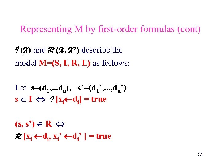
Representing M by first-order formulas (cont) I (X) and R (X, X’) describe the model M=(S, I, R, L) as follows: Let s=(d 1, . . . dn), s’=(d 1’, . . . , dn’) s I I [xi di] = true (s, s’) R R [xi di, xi’ di’ ] = true 53

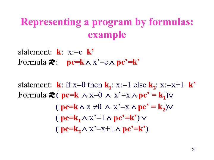
Representing a program by formulas: example statement: k: x: =e k’ Formula R : pc=k x’=e pc’=k’ statement: k: if x=0 then k 1: x: =1 else k 2: x: =x+1 k’ Formula R: ( pc=k x=0 x’=x pc’ = k 1) ( pc=k x 0 x’=x pc’ = k 2) ( pc=k 1 x’=1 pc’=k’) ( pc=k 2 x’=x+1 pc’=k’) 54

Given a formula over variables x 1, . . . , xk [ ] (x 1 A, . . . , xk. A) = x 1, . . . , xk ( h(x 1)= x 1 A . . . h(xk)= xk. A (x 1, . . . , xk) ) Let I (X) and R (X, X’) be the formulas describing M. Then [I (X) ] and [R (X, X’)] describe Mr Note: [I (X) ] and [R (X, X’)] are formulas over abstract variables 55

Problem: Given [I (X) ] and [R (X, X’)], in order to determine if sr Ir, we need to find a state s I (a satisfying assignment for I (X)) so that h(s) = sr. Similarly, for (sr, tr) Rr we look for a satisfying assignment for R (X, X’) This is a difficult task due to the size and complexity of the two formulas 56

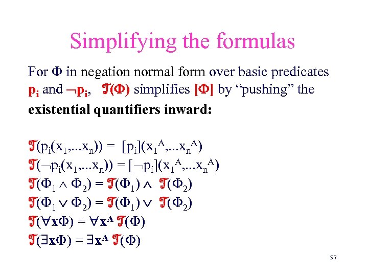
Simplifying the formulas For in negation normal form over basic predicates pi and pi, T( ) simplifies [ ] by “pushing” the existential quantifiers inward: T(pi(x 1, . . . xn)) = [pi](x 1 A, . . . xn. A) T( pi(x 1, . . . xn)) = [ pi](x 1 A, . . . xn. A) T( 1 2) = T( 1) T( 2) T( x ) = x. A T( ) 57

Approximation model Theorem: [ ] T( ) In particular, [I ] T(I ) and [R ] T(R ) Corollary: The approximation model Ma, defined by T(I ) and T(R ) satisfies: Ma Mr M by the simulation preorder 58

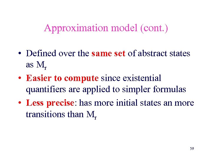
Approximation model (cont. ) • Defined over the same set of abstract states as Mr • Easier to compute since existential quantifiers are applied to simpler formulas • Less precise: has more initial states an more transitions than Mr 59

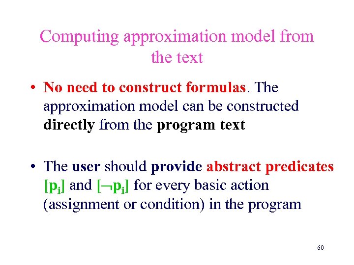
Computing approximation model from the text • No need to construct formulas. The approximation model can be constructed directly from the program text • The user should provide abstract predicates [pi] and [ pi] for every basic action (assignment or condition) in the program 60

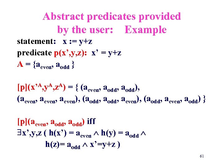
Abstract predicates provided by the user: Example statement: x : = y+z predicate p(x’, y, z): x’ = y+z A = {aeven, aodd } [p](x’A, y. A, z. A) = { (aeven, aodd), (aeven, aeven), (aodd, aeven, aodd) } [p](aeven, aodd) iff x’, y, z ( h(x’) = aeven h(y) = aodd h(z)= aodd x’=y+z ) 61

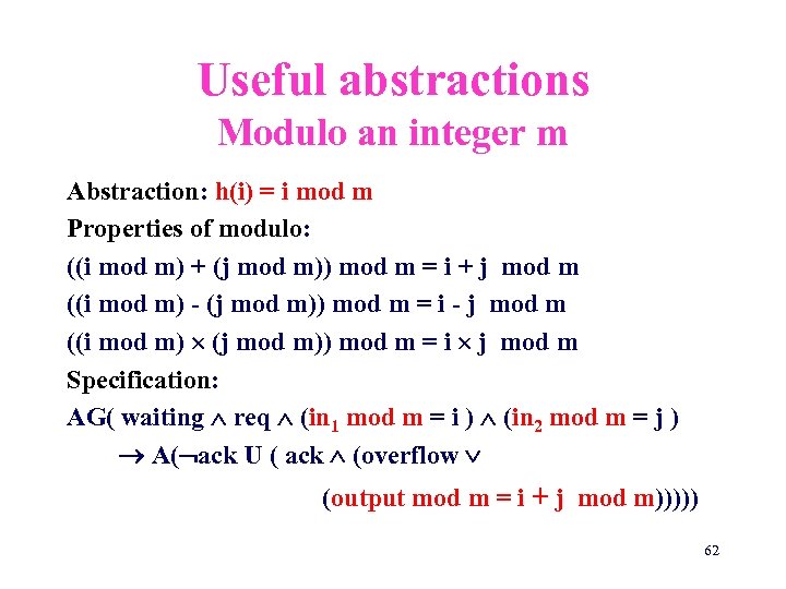
Useful abstractions Modulo an integer m Abstraction: h(i) = i mod m Properties of modulo: ((i mod m) + (j mod m)) mod m = i + j mod m ((i mod m) - (j mod m)) mod m = i - j mod m ((i mod m) (j mod m)) mod m = i j mod m Specification: AG( waiting req (in 1 mod m = i ) (in 2 mod m = j ) A( ack U ( ack (overflow (output mod m = i + j mod m))))) 62

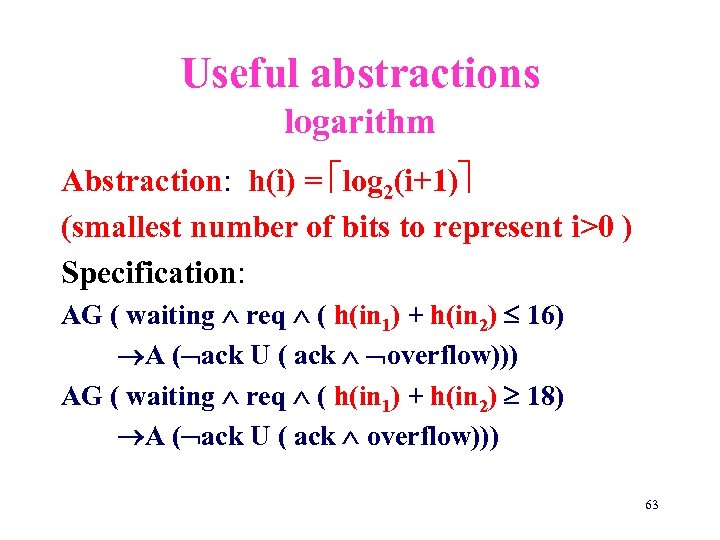
Useful abstractions logarithm Abstraction: h(i) = log 2(i+1) (smallest number of bits to represent i>0 ) Specification: AG ( waiting req ( h(in 1) + h(in 2) 16) A ( ack U ( ack overflow))) AG ( waiting req ( h(in 1) + h(in 2) 18) A ( ack U ( ack overflow))) 63

Counterexample-guided refinement Goal: • To produce abstraction automatically • To use counter example in order to refine the abstraction E. Clarke, O. Grumberg, S. Jha, Y. Lu, and H. Veith. Counterexample-guided abstraction Refinement, CAV’ 00 64

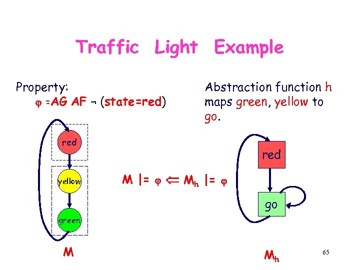
Traffic Light Example Property: =AG AF ¬ (state=red) Abstraction function h maps green, yellow to go. red yellow red M |= Mh |= go green M Mh 65

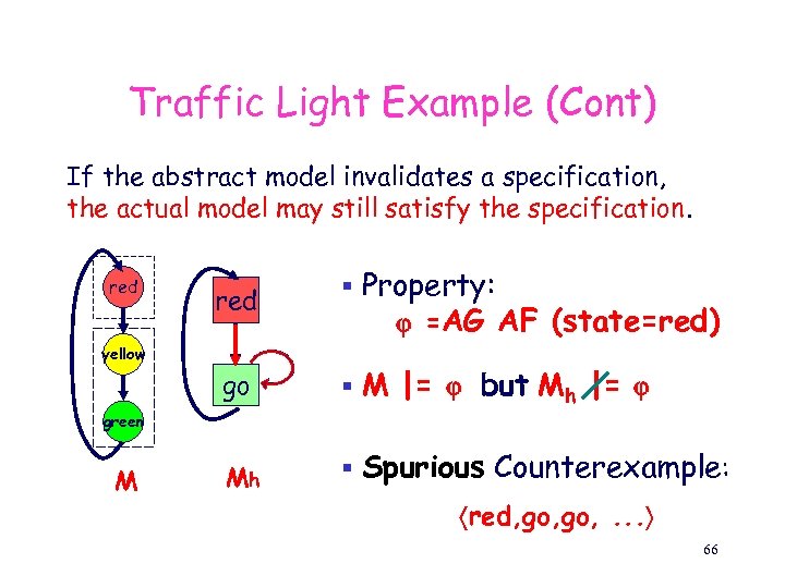
Traffic Light Example (Cont) If the abstract model invalidates a specification, the actual model may still satisfy the specification. red § Property: =AG AF (state=red) go red § M |= but Mh |= Mh § Spurious Counterexample: yellow green M red, go, . . . 66

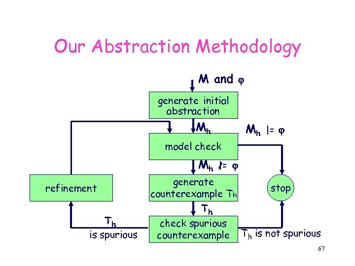
Our Abstraction Methodology M and generate initial abstraction Mh Mh |= model check Mh refinement Th is spurious |= generate counterexample Th Th check spurious counterexample stop Th is not spurious 67

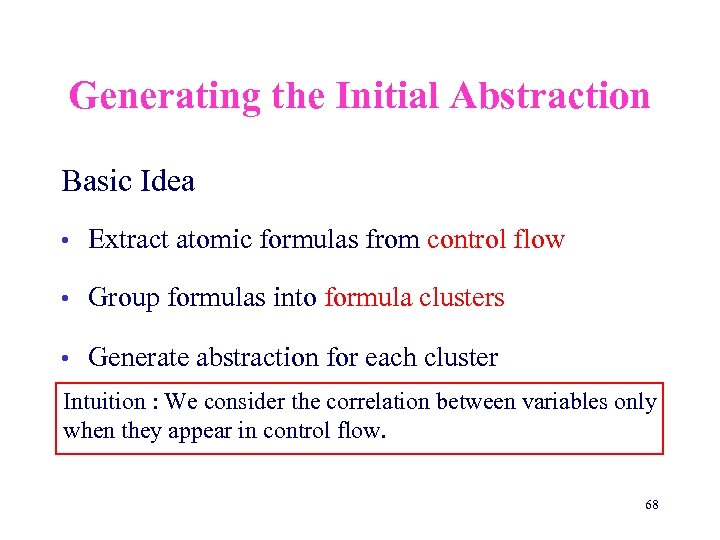
Generating the Initial Abstraction Basic Idea • Extract atomic formulas from control flow • Group formulas into formula clusters • Generate abstraction for each cluster Intuition : We consider the correlation between variables only when they appear in control flow. 68

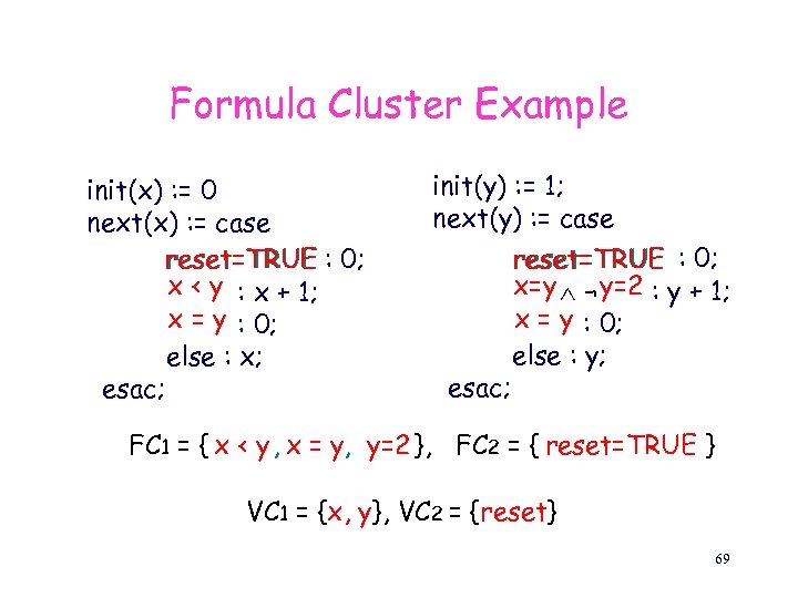
Formula Cluster Example init(x) : = 0 next(x) : = case reset=TRUE : 0; x < y : x + 1; x = y : 0; else : x; esac; init(y) : = 1; next(y) : = case esac; reset=TRUE : 0; x=y ¬ y=2 : y + 1; x = y : 0; else : y; FC 1 = { x < y , x = y, y=2 }, FC 2 = { reset=TRUE } VC 1 = {x, y}, VC 2 = {reset} 69

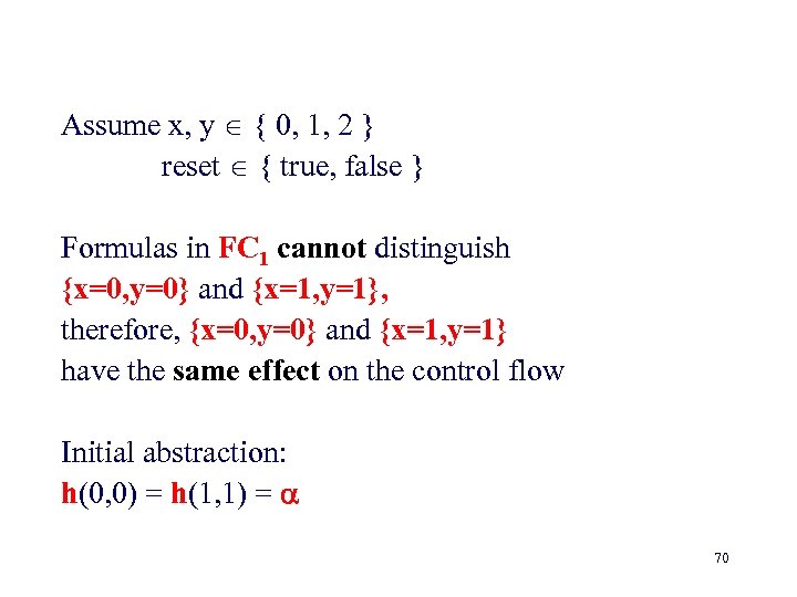
Assume x, y { 0, 1, 2 } reset { true, false } Formulas in FC 1 cannot distinguish {x=0, y=0} and {x=1, y=1}, therefore, {x=0, y=0} and {x=1, y=1} have the same effect on the control flow Initial abstraction: h(0, 0) = h(1, 1) = 70

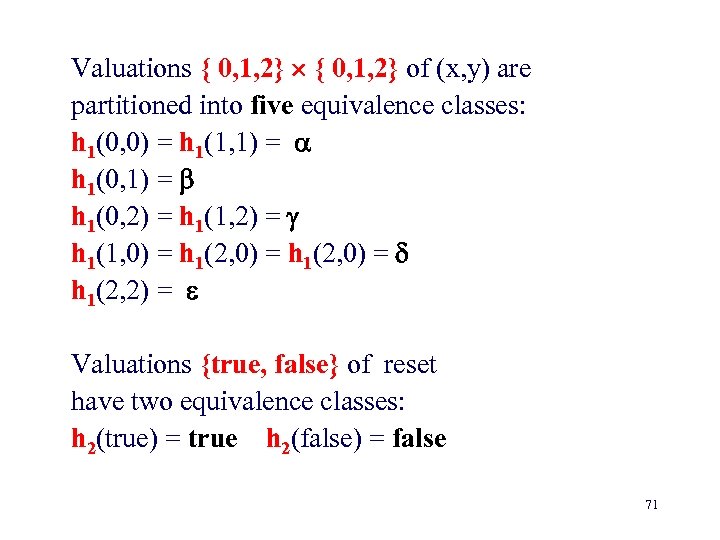
Valuations { 0, 1, 2} of (x, y) are partitioned into five equivalence classes: h 1(0, 0) = h 1(1, 1) = h 1(0, 2) = h 1(1, 2) = h 1(1, 0) = h 1(2, 0) = h 1(2, 2) = Valuations {true, false} of reset have two equivalence classes: h 2(true) = true h 2(false) = false 71

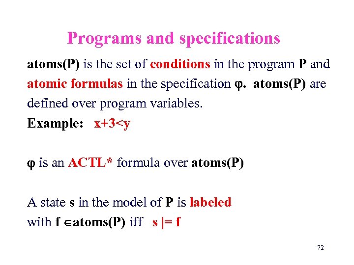
Programs and specifications atoms(P) is the set of conditions in the program P and atomic formulas in the specification . atoms(P) are defined over program variables. Example: x+3<y is an ACTL* formula over atoms(P) A state s in the model of P is labeled with f atoms(P) iff s |= f 72

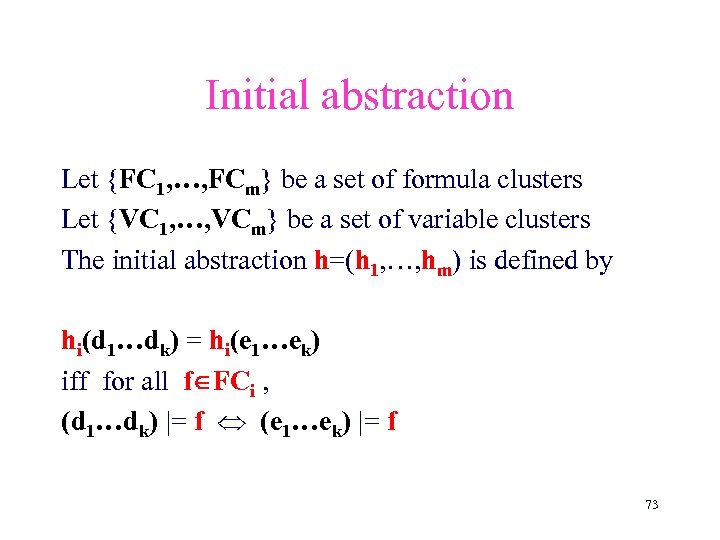
Initial abstraction Let {FC 1, …, FCm} be a set of formula clusters Let {VC 1, …, VCm} be a set of variable clusters The initial abstraction h=(h 1, …, hm) is defined by hi(d 1…dk) = hi(e 1…ek) iff for all f FCi , (d 1…dk) |= f (e 1…ek) |= f 73

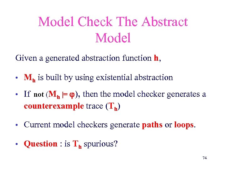
Model Check The Abstract Model Given a generated abstraction function h, • Mh is built by using existential abstraction • If not (Mh |= ), then the model checker generates a counterexample trace (Th) • Current model checkers generate paths or loops. • Question : is Th spurious? 74

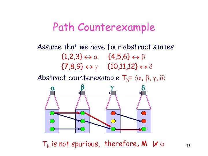
Path Counterexample Assume that we have four abstract states {1, 2, 3} {4, 5, 6} {7, 8, 9} {10, 11, 12} Abstract counterexample Th= , , , Th is not spurious, therefore, M |= 75

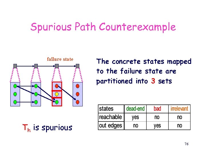
Spurious Path Counterexample failure state The concrete states mapped to the failure state are partitioned into 3 sets Th is spurious 76

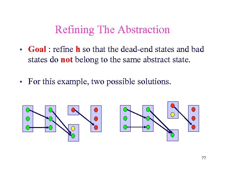
Refining The Abstraction • Goal : refine h so that the dead-end states and bad states do not belong to the same abstract state. • For this example, two possible solutions. 77

General Refinement Problem The optimal refinement is hard to find • Coarser refinements are safer • • the refined abstract machine is still small • Theorem: Finding the coarsest refinement is NP-hard. • Heuristic : Treat all the irrelevant states as bad states • in practice, this works very well 78

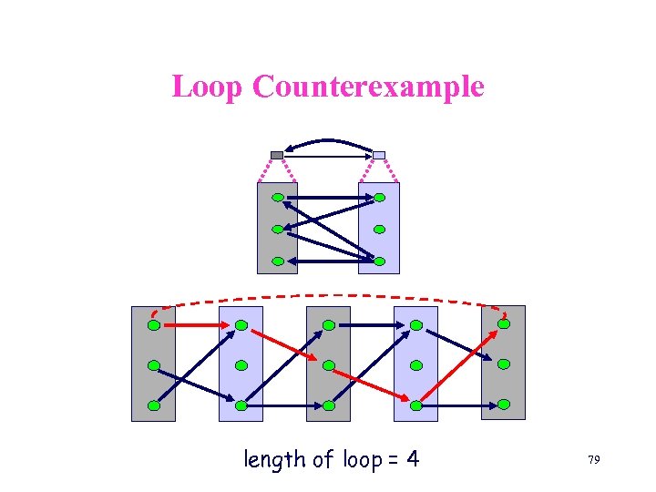
Loop Counterexample length of loop = 4 79

Loop Counterexample (cont) Important observations • The size of a concrete loop may be different from the abstract loop • An abstract loop may correspond to several concrete loops • Naïve unwinding may be exponential 80

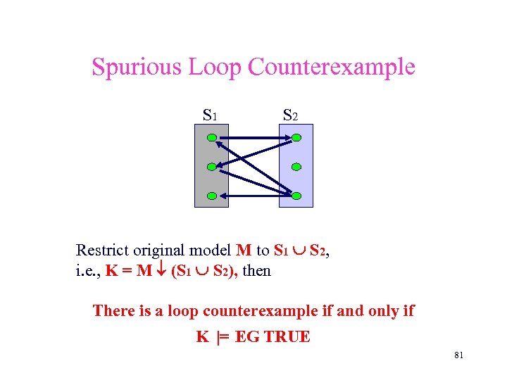
Spurious Loop Counterexample S 1 S 2 Restrict original model M to S 1 S 2, i. e. , K = M (S 1 S 2), then There is a loop counterexample if and only if K |= EG TRUE 81

Spurious Loop Counterexample • If an abstract loop counterexample is spurious, loop unwinding will reach empty set • Let Tunwind be the unwound loop by |S 1| times. • Theorem: The loop counterexample is spurious iff Tunwind is spurious. Use refinement algorithm for path counterexample! 82

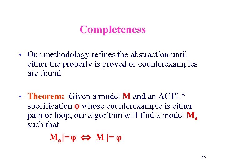
Completeness • Our methodology refines the abstraction until either the property is proved or counterexamples are found • Theorem: Given a model M and an ACTL* specification whose counterexample is either path or loop, our algorithm will find a model Ma such that Ma |= M |= 83

Experiment : Fujitsu Design The multimedia processor is very complicated • Description includes 61, 500 lines of Verilog code • Manual abstraction by Fujitsu engineers reduces the code to 10, 600 lines with 500 registers • We translated this abstracted code into 9, 500 lines of SMV code 84

Experiment (cont. ) We tried to verify this using state-of-art model checkers • Nu. SMV+COI cannnot verify the design • Bwolen Yang’s SMV cannot verify the design • Our approach abstracted 144 symbolic variables, used 3 refinement steps, and found a bug 85

Abstract Interpretation We show abstractions preserving temporal logics can be defined within the framework of abstract interpretation D. Dams, R. Gerth, O. Grumberg, Abstract interpretation of reactive systems, TOPLAS Vol. 19, No. 2, March 1997. 86

Abstract interpretation (cont. ) We define abstractions that preserve: – Existential properties (ECTL*) – Universal properties (ACTL*) – Both (CTL*) We define: • Canonical abstraction that preserves maximum number of temporal properties • Approximations 87

Abstract interpretation (cont. ) Using abstract interpretation we can obtain abstract models which are more precise (and therefore preserve more properties) than the existential abstraction presented before 88

The Abstract Interpretation Framework • Developed by Cousot & Cousot for compiler optimization • Constructs an abstract model directly from the program text • Classical abstract interpretations preserve properties of states. Here we are interested in properties of computations 89

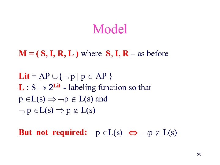
Model M = ( S, I, R, L ) where S, I, R – as before Lit = AP { p | p AP } L : S 2 Lit - labeling function so that p L(s) p L(s) and p L(s) p L(s) But not required: p L(s) p L(s) 90

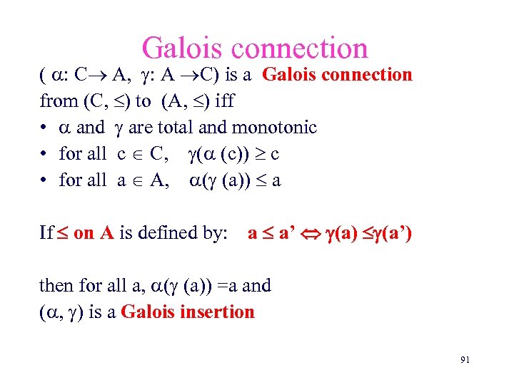
Galois connection ( : C A, : A C) is a Galois connection from (C, ) to (A, ) iff • and are total and monotonic • for all c C, ( (c)) c • for all a A, ( (a)) a If on A is defined by: a a’ (a) (a’) then for all a, ( (a)) =a and ( , ) is a Galois insertion 91

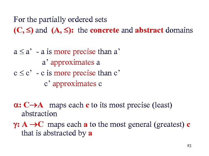
For the partially ordered sets (C, ) and (A, ): the concrete and abstract domains a a’ - a is more precise than a’ a’ approximates a c c’ - c is more precise than c’ c’ approximates c : C A maps each c to its most precise (least) abstraction : A C maps each a to the most general (greatest) c that is abstracted by a 92

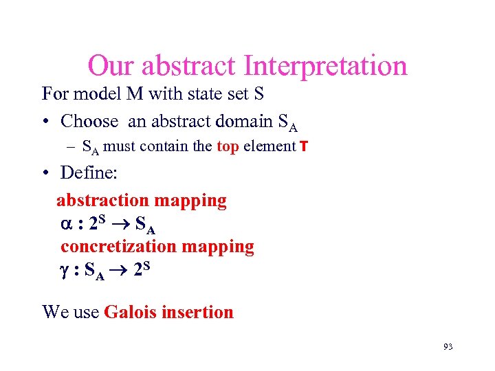
Our abstract Interpretation For model M with state set S • Choose an abstract domain SA – SA must contain the top element T • Define: abstraction mapping : 2 S S A concretization mapping : SA 2 S We use Galois insertion 93

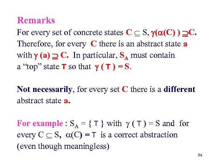
Remarks For every set of concrete states C S, ( (C) ) C. Therefore, for every C there is an abstract state a with (a) C. In particular, SA must contain a “top” state T so that ( T ) = S. Not necessarily, for every set C there is a different abstract state a. For example : SA = { T } with ( T ) = S and for every C S, (C) = T is a correct abstraction (even though meaningless) 94

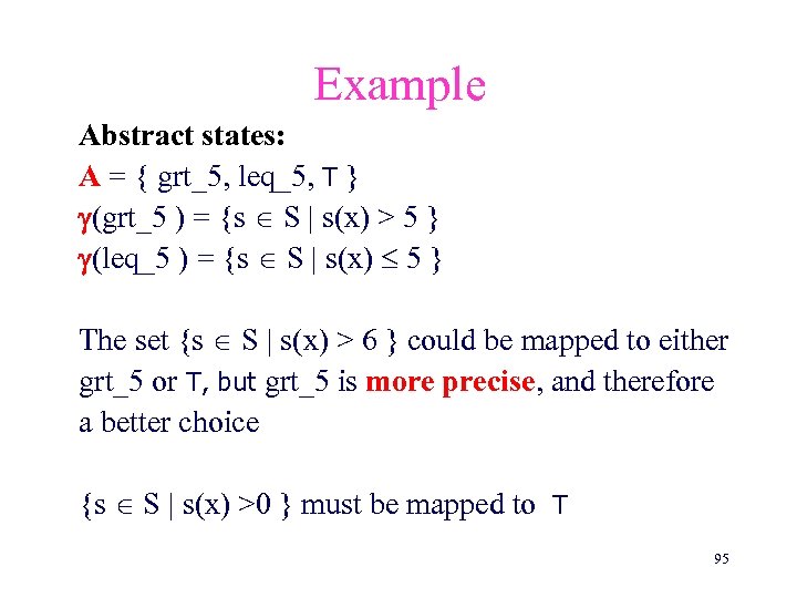
$Example Abstract states: A = { grt_5, leq_5, T } (grt_5 ) = {s$

Example Abstract states: A = { grt_5, leq_5, T } (grt_5 ) = {s S | s(x) > 5 } (leq_5 ) = {s S | s(x) 5 } The set {s S | s(x) > 6 } could be mapped to either grt_5 or T, but grt_5 is more precise, and therefore a better choice {s S | s(x) >0 } must be mapped to T 95

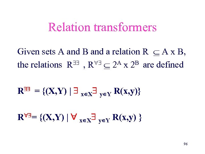
Relation transformers Given sets A and B and a relation R A x B, the relations R , R 2 A x 2 B are defined R = {(X, Y) | x X y Y R(x, y)} R = {(X, Y) | x X y Y R(x, y) } 96

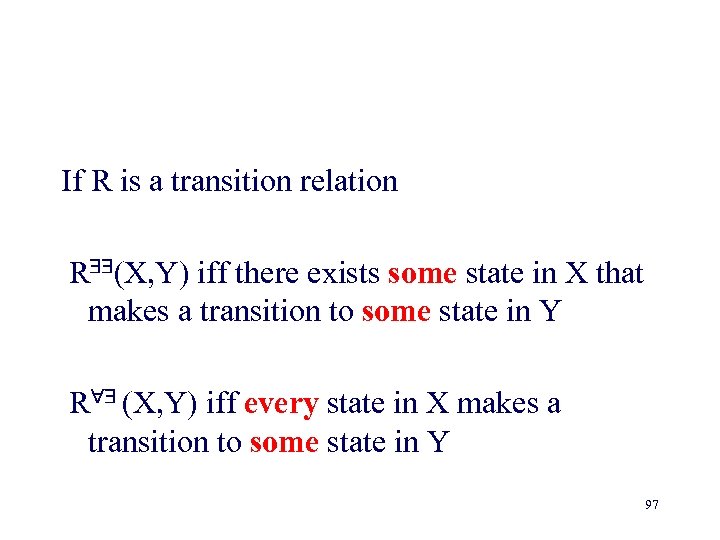
If R is a transition relation R (X, Y) iff there exists some state in X that makes a transition to some state in Y R (X, Y) iff every state in X makes a transition to some state in Y 97

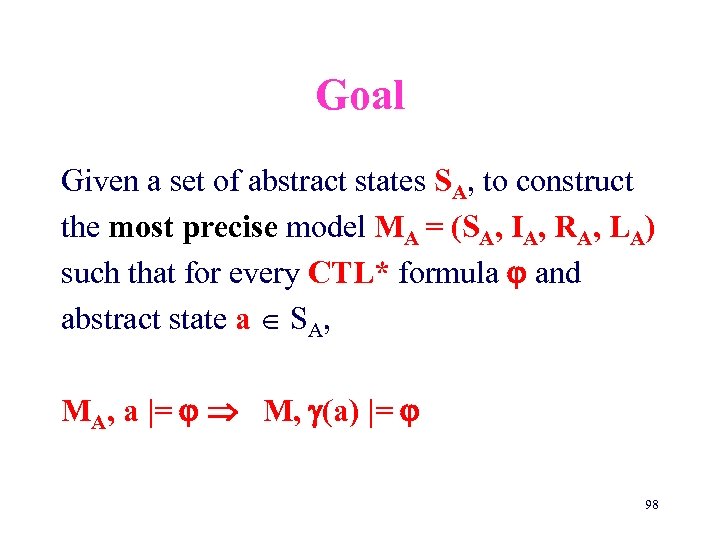
Goal Given a set of abstract states SA, to construct the most precise model MA = (SA, IA, RA, LA) such that for every CTL* formula and abstract state a SA, MA, a |= M, (a) |= 98

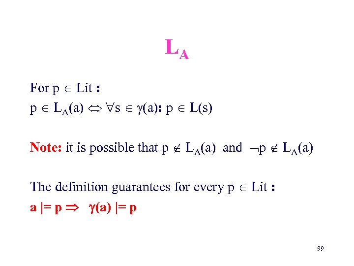
LA For p Lit : p LA(a) s (a): p L(s) Note: it is possible that p LA(a) and p LA(a) The definition guarantees for every p Lit : a |= p (a) |= p 99

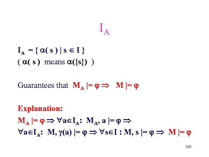
IA IA = { ( s ) | s I } ( ( s ) means ({s}) ) Guarantees that MA |= M |= Explanation: MA |= a IA: MA, a |= a IA: M, (a) |= s I : M, s |= M |= 100

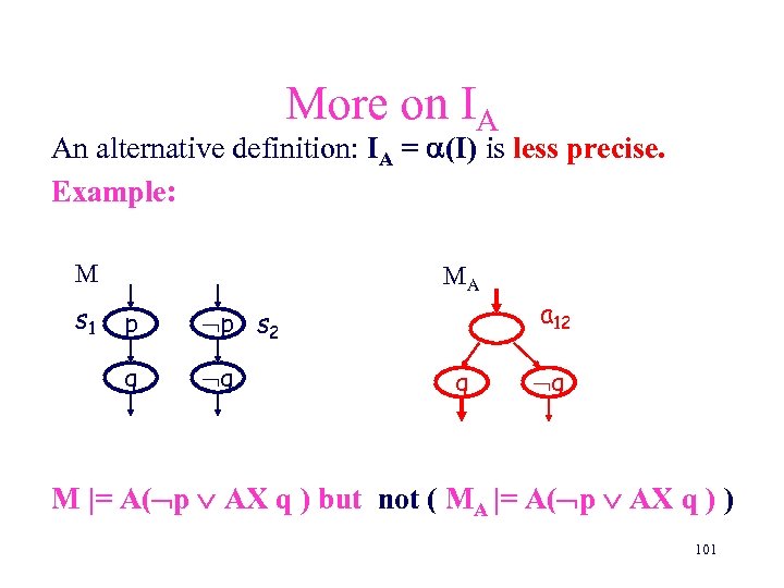
More on IA An alternative definition: IA = (I) is less precise. Example: M s 1 MA p p s 2 q q q a 12 q M |= A( p AX q ) but not ( MA |= A( p AX q ) ) 101

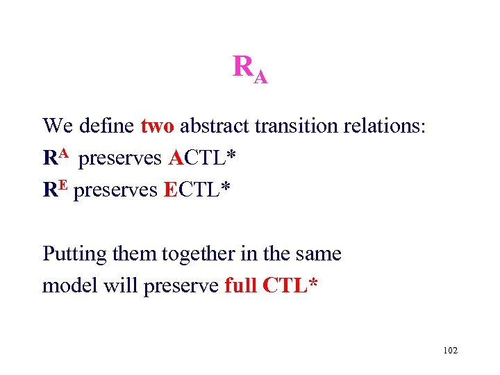
RA We define two abstract transition relations: RA preserves ACTL* RE preserves ECTL* Putting them together in the same model will preserve full CTL* 102

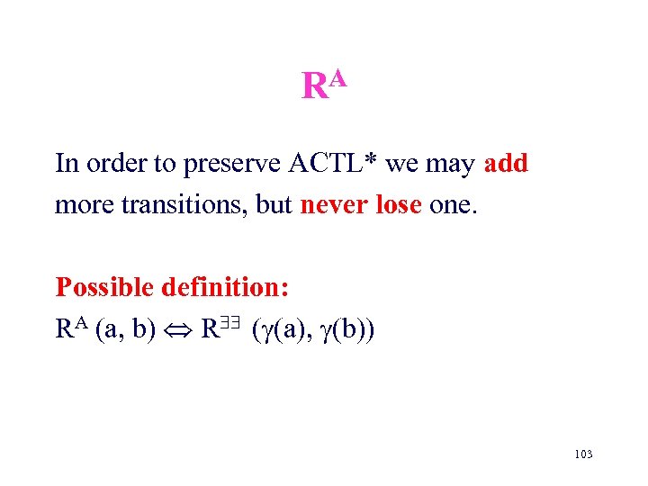
A R In order to preserve ACTL* we may add more transitions, but never lose one. Possible definition: RA (a, b) R ( (a), (b)) 103

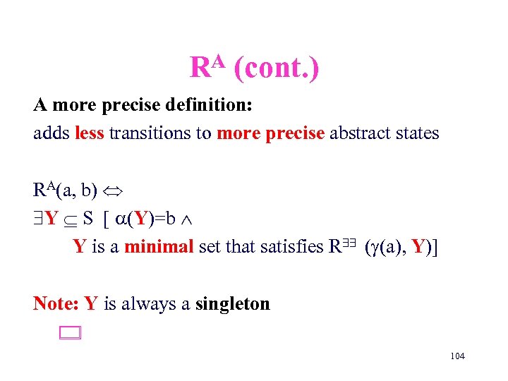
A R (cont. ) A more precise definition: adds less transitions to more precise abstract states RA(a, b) Y S [ (Y)=b Y is a minimal set that satisfies R ( (a), Y)] Note: Y is always a singleton 104

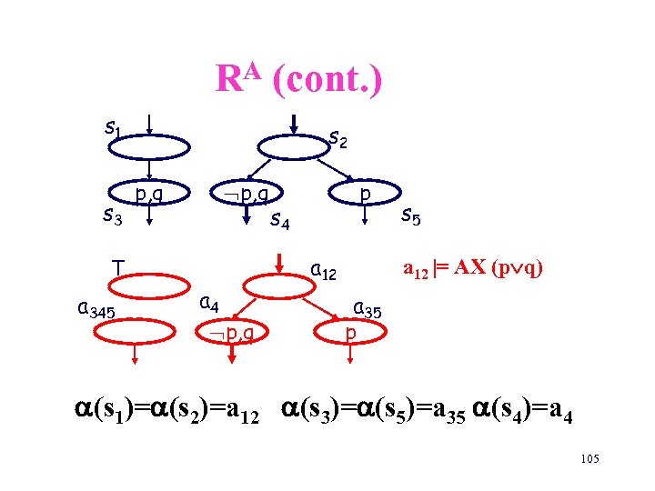
A R (cont. ) s 1 s 3 s 2 p, q T a 345 a 4 p, q p s 4 a 12 s 5 a 12 |= AX (p q) a 35 p (s 1)= (s 2)=a 12 (s 3)= (s 5)=a 35 (s 4)=a 4 105

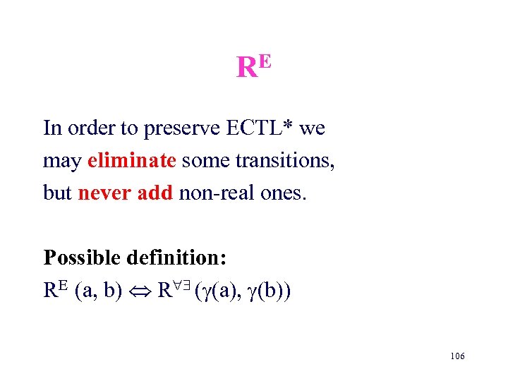
E R In order to preserve ECTL* we may eliminate some transitions, but never add non-real ones. Possible definition: RE (a, b) R ( (a), (b)) 106

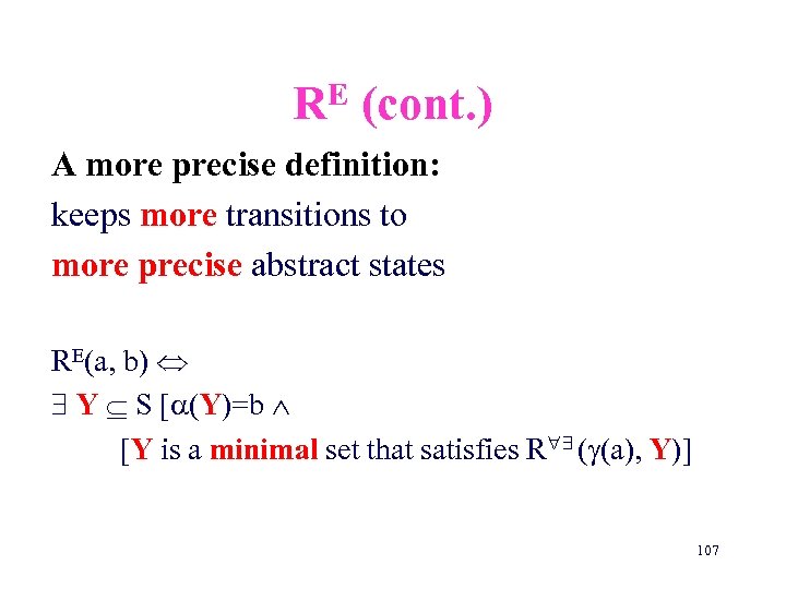
E R (cont. ) A more precise definition: keeps more transitions to more precise abstract states RE(a, b) Y S [ (Y)=b [Y is a minimal set that satisfies R ( (a), Y)] 107

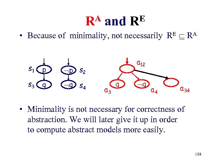
RA and RE • Because of minimality, not necessarily RE RA s 1 p p s 2 s 3 q q s 4 a 12 a 3 q q a 4 a 34 • Minimality is not necessary for correctness of abstraction. We will later give it up in order to compute abstract models more easily. 108

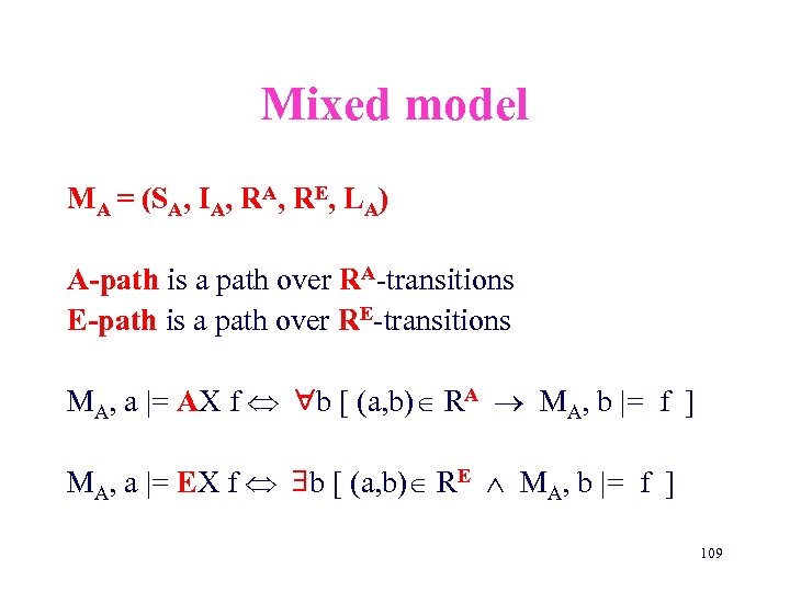
Mixed model MA = (SA, IA, RE, LA) A-path is a path over RA-transitions E-path is a path over RE-transitions MA, a |= AX f b [ (a, b) RA MA, b |= f ] MA, a |= EX f b [ (a, b) RE MA, b |= f ] 109

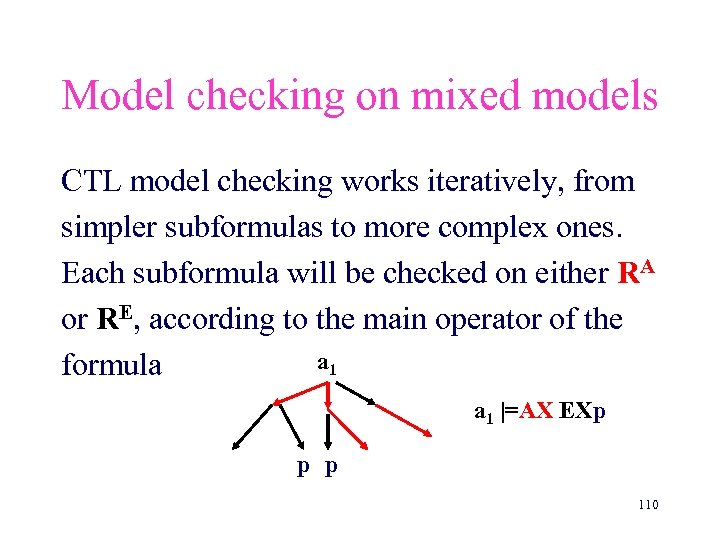
Model checking on mixed models CTL model checking works iteratively, from simpler subformulas to more complex ones. Each subformula will be checked on either RA or RE, according to the main operator of the a 1 formula a 1 |=AX EXp p p 110

We have constructed MA, which given SA, , is the best model satisfying for every in CTL* MA |= M |= If not ( MA |= ) then we can check whether MA |= . If neither holds then SA is too coarse to give the answer. 111

Approximations As in other abstractions: • We would like to construct the abstraction directly from the program text • Best abstraction is too difficult to compute • We therefore construct approximation to the abstraction 112

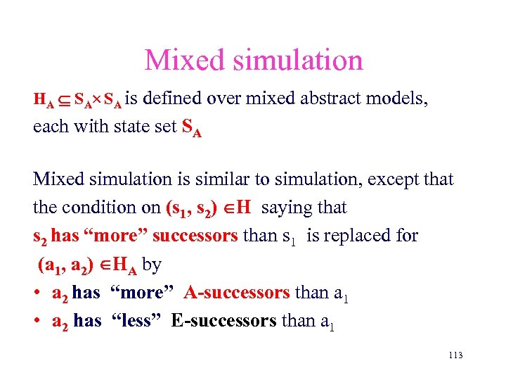
Mixed simulation HA SA SA is defined over mixed abstract models, each with state set SA Mixed simulation is similar to simulation, except that the condition on (s 1, s 2) H saying that s 2 has “more” successors than s 1 is replaced for (a 1, a 2) HA by • a 2 has “more” A-successors than a 1 • a 2 has “less” E-successors than a 1 113

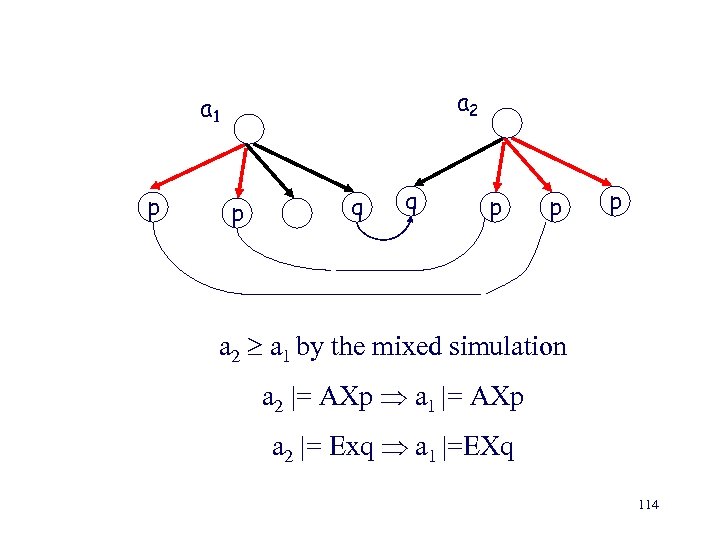
a 2 a 1 p p q q p p p a 2 a 1 by the mixed simulation a 2 |= AXp a 1 |= AXp a 2 |= Exq a 1 |=EXq 114

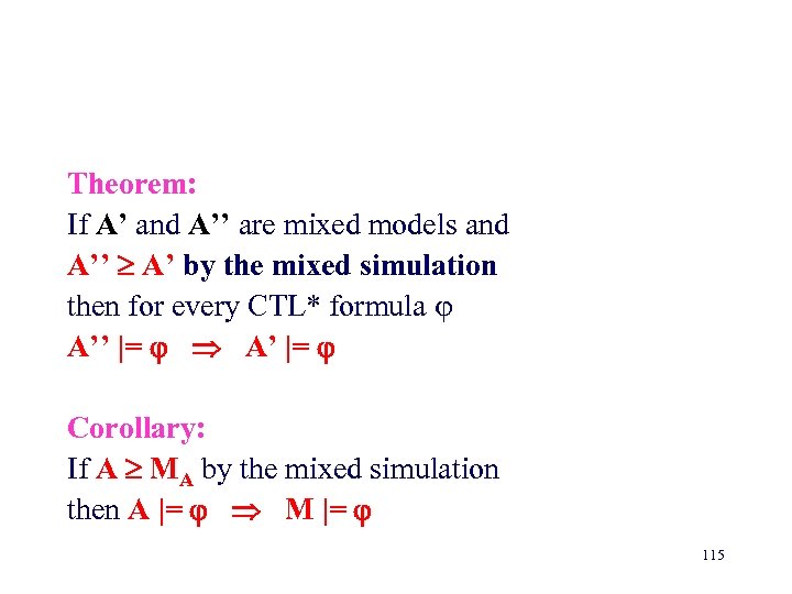
Theorem: If A’ and A’’ are mixed models and A’’ A’ by the mixed simulation then for every CTL* formula A’’ |= A’ |= Corollary: If A MA by the mixed simulation then A |= M |= 115

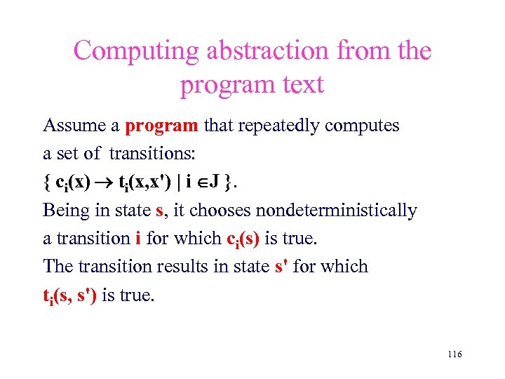
Computing abstraction from the program text Assume a program that repeatedly computes a set of transitions: { ci(x) ti(x, x') | i J }. Being in state s, it chooses nondeterministically a transition i for which ci(s) is true. The transition results in state s' for which ti(s, s') is true. 116

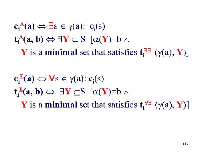
ci. A(a) s (a): ci(s) ti. A(a, b) Y S [ (Y)=b Y is a minimal set that satisfies ti ( (a), Y)] ci. E(a) s (a): ci(s) ti. E(a, b) Y S [ (Y)=b Y is a minimal set that satisfies ti ( (a), Y)] 117

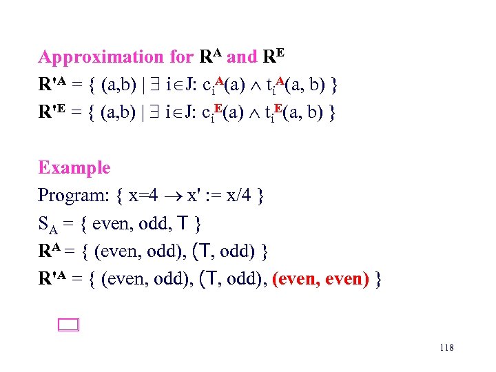
Approximation for RA and RE R'A = { (a, b) | i J: ci. A(a) ti. A(a, b) } R'E = { (a, b) | i J: ci. E(a) ti. E(a, b) } Example Program: { x=4 x' : = x/4 } SA = { even, odd, T } RA = { (even, odd), (T, odd) } R'A = { (even, odd), (T, odd), (even, even) } 118

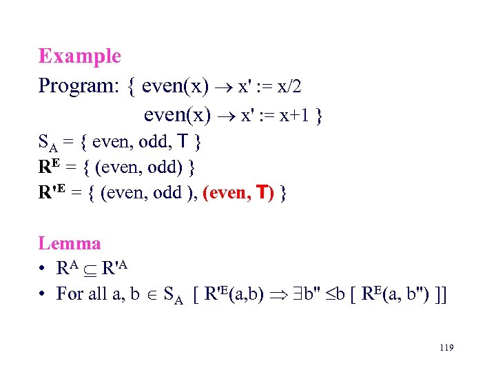
Example Program: { even(x) x' : = x/2 even(x) x' : = x+1 } SA = { even, odd, T } RE = { (even, odd) } R'E = { (even, odd ), (even, T) } Lemma • RA R'A • For all a, b SA [ R'E(a, b) b'' b [ RE(a, b'') ]] 119

Further approximation Give up minimality in the definition of ti. A and ti. E : Replace transition (a, b) by transition (a, b') with b b' by the mixed simulation. • Easier to compute from the program text. • Still preserves (possibly less) CTL* formulas. 120

State-of-the-art Abstraction F Abstract interpretation (Cousot & Cousot 77, Loiseaux & Graf & Sifakis & Bouajjani & Bensalem 95, Graf 94) F (Bi)-simulation reduction (Bouajjani & Fernandez & Halbwachs 90, Lee & Yannakakis 92, Fisler & Vardi 98, Bustan & Grumberg 00) F Formula-dependent equivalence (Aziz & Singhal & Shiple & Sangiovanni-Vincentelli 94) F Compositional minimization (Aziz & Singhal & Swamy & Brayton 94) 121

State-of-the-art Abstraction (Cont) F Uninterpreted functions (Burch & Dill 94, Berzin & Biere & Clarke & Zhu 98, Bryant & German & Velve 99) F Abstraction and refinement (Dams & Gerth & Grumberg 93, Kurshan 94, Balarin & Sangiovanni-Vincentelli 93, Lind-Nielsen & Andersen 99) F Predicate abstraction and Theorem proving (Das & Dill & Park 99, Graf & Saidi 97, Uribe 99) 122

The End 123