4ecf6c6c9667e53e439336ddcc1b51f9.ppt
- Количество слайдов: 76


Model Based Computer Vision Arun Agarwal University of Hyderabad aruncs@uohyd. ernet. in

Examples of applications • Outdoor Scenes, Block World, Real World • Natural Scenes • Biometrics • Autonomous Land Vehicle • Aerial Imaging (Airport Scenes) • Face recognition, verification, retrieval. • Finger prints recognition. • Diagnostic systems • Medical diagnosis: X-Ray. • Military applications • Automated Target Recognition (ATR). • Image segmentation and analysis (recognition from aerial or satelite photographs).
 Labeled Objects High level I U Features, attributes")
Hierarchy of Image Understanding System (IUS) Labeled Objects High level I U Features, attributes and relationships S Images Input image Intermediate Level Low level

DESCRIPTION SEMANTIC INTERPRETATION SCENE MODELS SYMBOLIC REPRESENTATION REGION / EDGE FEATURE EXTRACTION IMAGE BLOCK DIAGRAM OF BOTTOM-UP APPROACH

SCENE DESCRIPTION INTERPRETATION MODEL SYMBOLIC REPRESENTATION REGION / EDGE FEATURE EXTRACTION IMAGE TOP-DOWN APPROACH

SCENE DESCRIPTION INTERPRETATION MODEL SYMBOLIC REPRESENTATION REGION / EDGE FEATURE EXTRACTION IMAGE REPRESENTATIVE BLOCK DIAGRAM OF TOP DOWN BOTTOM UP APPROACH

METHODS KNOWLEDGE SOURCES SCHEDULER BLACKBOARD MODEL APPROACH

Approaches z Statistical Model: based on underlying statistical model of patterns and pattern classes. z Syntactic Model: pattern classes represented by means of formal structures as grammars, automata, strings, graphs, constraint matrix etc. z Structural Model: knowledge base,

Statistical PR

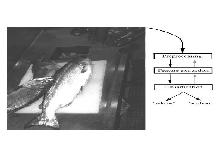
An Example z“Sorting incoming Fish on a conveyor according to species using optical sensing” Sea bass Species Salmon

z Problem Analysis y. Set up a camera and take some sample images to extract features x. Length x. Lightness x. Width x. Number and shape of fins x. Position of the mouth, etc… x. This is the set of all suggested features to explore for use in our classifier!

z Preprocessing y. Use a segmentation operation to isolate fishes from one another and from the background z. Information from a single fish is sent to a feature extractor whose purpose is to reduce the data by measuring certain features z. The features are passed to a classifier

z. Classification y. Select the length of the fish as a possible feature for discrimination
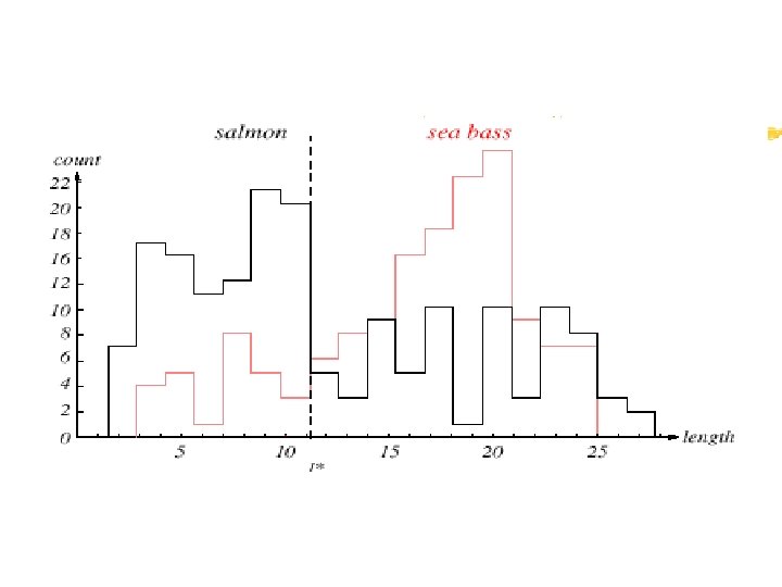

The length is a poor feature alone! Select the lightness as a possible feature.
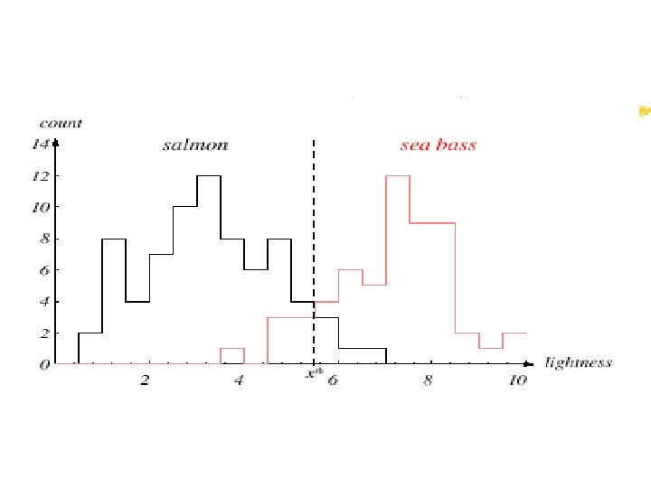

z. Threshold decision boundary and cost relationship y. Move our decision boundary toward smaller values of lightness in order to minimize the cost (reduce the number of sea bass that are classified salmon!) Task of decision theory

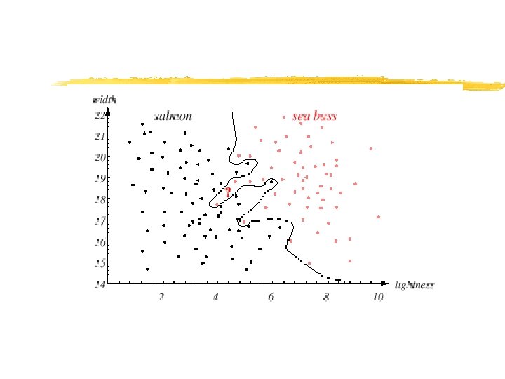
z. Adopt the lightness and add the width of the fish Fish x. T = [x 1, x 2] Lightness Width
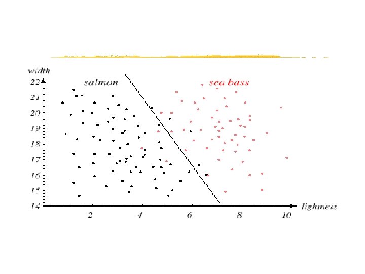

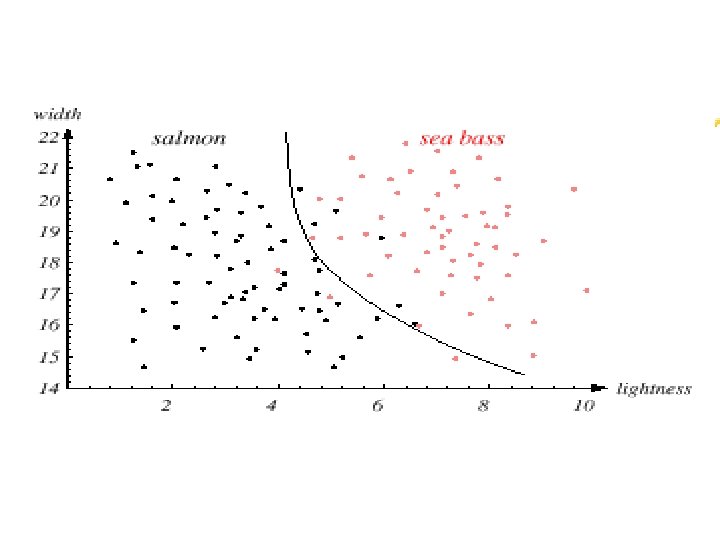
z. We might add other features that are not correlated with the ones we already have. A precaution should be taken not to reduce the performance by adding such “noisy features” z. Ideally, the best decision boundary should be the one which provides an optimal performance such as in the following figure:
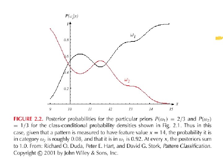

z Decision given the posterior probabilities X is an observation for which: if P( 1 | x) > P( 2 | x) if P( 1 | x) < P( 2 | x) True state of nature = 1 True state of nature = 2 Therefore: whenever we observe a particular x, the probability of error is : P(error | x) = P( 1 | x) if we decide 2 P(error | x) = P( 2 | x) if we decide 1
")
z Minimizing the probability of error z Decide 1 if P( 1 | x) > P( 2 | x); otherwise decide 2 Therefore: P(error | x) = min [P( 1 | x), P( 2 | x)] (Bayes decision)

Optimal decision property “If the likelihood ratio exceeds a threshold value independent of the input pattern x, we can take optimal actions”

Syntactic PR

Syntactic Pattern Recognition Technique Syntactic Pattern Recognition consists of three major steps: Preprocessing which improves the quality of an image, e. g. filtering, enhancement, etc. Pattern representation which segments the picture and assigns the segments to the parts in the model Syntax picture which analysis recognizes the according to the syntactic model: once a grammar has been defined, some type of recognition device is required, the application of such a recognizer is called Parsing. Syntactic methods are best suited to problems with clear primitives and stable intermediate structures, with well defined and known alternative. A very important issue in syntactic pattern recognition is that of grammatical interface.

Block Diagram of a Syntactic Pattern Recognition System Input Pattern Preprocessing Segmentation Primitive Representation (and relation) Construction recognition Syntax Classification Analysis (Parsing) Recognition Training Patterns Primitive (and relation) selection Grammatical Interface Automata Construction

Grammar z Grammars can be classified to four categories according to their productions: z Unrestricted grammar z Context sensitive grammar z Context free grammar z Regular grammar z Depending on the options available at each stage of the rewriting process, a grammar can be classified as: z Deterministic z Non-deterministic z Stochastic
 Objects K FGL A J H I Object B")
SEMANTIC PRIMITIVES Scene Background (Subpattern) Objects K FGL A J H I Object B Object A (Subpatterns) Floor L Wall K B F G Face H (Subpatterns) Face I Face J Hierarchical Structures

An Example Pattern Primitives a unit 3 units a a b c d Tree Structure Rectangle a d b c c c 2 units a + a + b+ c + c + d +d String form: aaabbcccdd More explicitly: ‘+’ head-to-tail concatenation a+a+a+b+b+c+c+c+d+d

An Example Pattern and its Structural Description Pattern Subpattern c + d + a + b b + c + c Pattern primitives

For this approach to be advantageous the simplest subpattern selected called pattern primitives, should be much easier to recognize the patterns themselves. Composition Of primitives patterns Accomplish by Grammar Once the primitives of the pattern are identified than recognition is accomplished by performing a syntax analysis or parsing.

a b An Exhaustive Example d a b b a b c e c c b a b b d b b a telocentric Chromosome Submedian Chromosome Context-free grammar G = (VN, VT, P {<Submedian Chromosome>, <telocentric Chromosome>}) Where VN = {<Submedian Chromosome>, <telocentric Chromosome>, <arm pair>, <left part>, <right part>, <arm>, <side>, <bottom>} VT = a b c d e

Productions {P}: <Submedian Chrom. > <telocentric Chrom. > <arm pair> <left part> <right part> <bottom> <side> <arm> <arm pair> <bottom> <arm pair> <side> <arm> <right part> <left part> <arm> c c <arm> b <bottom> b e b <side> b b d b <arm> b a

Now Given String babcbabd BOTTOM-UP PARSING OR DATA DRIVEN Submedian Chromosome arm pair left part arm arm arm b a arm side arm arm b c b a b d b a b c b a b d side

Structural PR

Example: Outdoor Scenes What is Image Understanding? Image Understanding is a process of understanding the image by identifying the objects in a scene and establishing relationships among the objects. Image Understanding is the task- oriented reconstruction and interpretation of a scene by means of images.
![Different Image understanding Systems z VISION [C. C. Parma] (1980) z ARGOS [Steven M.](https://present5.com/presentation/4ecf6c6c9667e53e439336ddcc1b51f9/image-41.jpg "Different Image understanding Systems z VISION [C. C. Parma] (1980) z ARGOS [Steven M.")
Different Image understanding Systems z VISION [C. C. Parma] (1980) z ARGOS [Steven M. Rubin] (1978) z ACRONYM [R. A. Brooks] (1981) z MOSAIC [T. Herman and T. Kanade] (1984) z SPAM [D. M. Mc. Keown] (1985) z SCERPO [Lowe] (1987) z SIGMA [Takashi and Vincent Hwang] (1990) z Knowledge-Based Medical Image Interpretation [Darryl N. Davis] (1991) and many more …
 of agrarian nation N TOP")
An example: Labeling of a very small picture (satellite) of agrarian nation N TOP ALFALFA LEFT BARLEY CORN RIGHT BOTTOM Knowledge Network Assume satellite photograph: 4 2 pixels Some possible labelling of 4 2 pixels image given the constraints of the knowledge network ie 1 5 2 6 3 4 7 8 > 6000 possible labellings A A A B C A A B B C C B C B C A B B B A A A B B B C C B B A B B B C C A B B C B C B C C C
 (arbitrary) on (seldom) streets (S) houses (H) (at least one)")
Example 2: cars (c) (arbitrary) on (seldom) streets (S) houses (H) (at least one) (arbitrary) on (often) inters. , A 1 on (always) Junc. , adj. H 2 H 1 A 2 SCENE MODEL on adj A 2 above on adj A 1 on S 1 body same size above H 2 before above before adj Junc. adj luggage boat rear wheel H 1 C A 3 S 1 other areas (A) (at least two) adj S 2 front wheel A 3 INSTANCE OF THE MODEL pess. room hood OBJECT MODEL (CAR)
 Isomorphism (ii) Largest Clique Image How to match")
Given: Object Model Two Approaches: (i) Isomorphism (ii) Largest Clique Image How to match ?

HOUSE SCENE F ROAD SCENE . O O N O F DRIVEWAY NO. TREE HOUSE LIKE - A ROAD ON S GARAGE IDE CAR GUARDRAILS SCENE CLASSES TELEPHONE POLES
![ON YS A LW A ROADS (R) [AT LEAST ONE] ND HI N BE](https://present5.com/presentation/4ecf6c6c9667e53e439336ddcc1b51f9/image-46.jpg "ON YS A LW A ROADS (R) [AT LEAST ONE] ND HI N BE")
ON YS A LW A ROADS (R) [AT LEAST ONE] ND HI N BE TE OF AL AD W J AY S HOUSE (H) OFTEN [ARBITRARY] ADJACENT TO ROAD RAIL [ARBITRARY LENGTH] CO NN EC TIO N ON YS A LW A BEHIND ALWAYS TELEPHONE POLES CARS (C) [ARBITRARY] N Y O EL AR R OTHER AREAS [AT LEAST TWO] TREES [ARBITRARY] ON ALWAYS NETWORK OF GENERAL ROAD_SCENE

Segmentation Given input image is segmented into different regions by using different segmentation methods. 1. Cluster based segmentation • K-means clustering algorithm • Porter and Canagarajah Method • Validity Measure Method 2. Ohlander type segmentation 3. Comaniciu and Meer proposed Algorithm

By observing the results of above segmentation algorithms, segmented image obtained by Comaniciu and Meer proposed segmentation Algorithm is only used for further processing. Results obtained by Comaniciu and Meer proposed segmentation algorithm are. . Original Image Segmented Image

Feature Extraction Two types of features are extracted from the segmented regions. 1. Primary features: 2. These features calculation directly deals with image arrays. It includes Area, Mean intensities of R, G&B, contour length, mass centers, Minimum bounding rectangle(MBR) and etc. 3. 2. Secondary features : 4. These features are calculated from a set of primary features. It includes compactness of regions, linearity, normalized colors, Hue, saturation and intensity values and etc.
, g = G/(R+G+B), b = B/(R+G+B), Intensity =")
Formulae : r = R/(R+G+B), g = G/(R+G+B), b = B/(R+G+B), Intensity = (R+G+B)/3, Hue = arc tan 2(31/2(G-B), (2 R-G-B)), Saturation = 1 -3 min(r, g, b), Compactness = 4 (area)/(contour length)2, and many more…
")
X Y MAX Y MIN X MIN Y X MAX MINIMUM BOUNDING RECTANGLE (MBR) PERIMETER (P) AREA (A) AN IRREGULAR FIGURE
 X")
Y BOUNDARY CHAIN CODES TH 1 CONTRAST NG 2 LE 0 3 (a) X (b) KEY FEATURES OF BOUNDARY SEGMENTS Y LENGTH X END POINT KEY FEATURES OF LINE SEGMENTS

Image Synthesis An image is constructed from the primary and secondary features those are extracted in the earlier phase. This synthesized image is compared with the original image. Greater the similarities , better the extracted features and segmentation algorithm. Synthesized Image Original image

Scene Interpretation Module This scene interpretation Module includes various sub-modules. those are… 1. Outdoor Scene Knowledgebase • Knowledge Extraction • Knowledge Representation 2. Plan Generation 3. Relaxation Labeling 4. Image Interpretation

Outdoor Scene Knowledgebase Outdoor scene Knowledgebase contains all the knowledge about the scenes like raw picture data(RGB values, edges etc), features information, constraints on those features and etc. Knowledgebase for outdoor scenes is divided into 3 parts. 1. Knowledge Extraction • Region Features • Object Features • Binary object relations 2. Knowledge Representation • Image domain knowledge • Scene domain knowledge 3. Constraint Matrix Generation

Knowledge Extraction • Region Features: This relation is domain-independent, which includes region attributes such as region number, the three-color features, average intensity, centroid, area, minimum bounded rectangle, hue, saturation and linearity. • Object Features: This relation contains the object name as a domain, followed by a set of domain triplets, each of which contains the feature name, whether or not this feature has a veto, and acceptable variation for each of the feature. Features extracted for objects ‘Sky’, ‘Building’, ‘Tree’ and ‘Grass’ are Sky: R = [49, 154], G = [96, 194], B = [162, 239], Hue = [202, 218], Compactness = [0. 0853, 0. 8289], Linearity = [43. 038, 82. 1362].
![Grass: Hue = [71, 105], Compactness = [0. 0813, 0. 168], Linearity =](https://present5.com/presentation/4ecf6c6c9667e53e439336ddcc1b51f9/image-57.jpg "Grass: Hue = [71, 105], Compactness = [0. 0813, 0. 168], Linearity =")
Grass: Hue = [71, 105], Compactness = [0. 0813, 0. 168], Linearity = [39. 4317, 75. 77], R = [76, 141], G = [92, 166], B = [36, 101]. Tree: Hue = [51, 93], Compactness = [0. 002, 0. 3801], Linearity = [25. 965, 35. 963], R = [49, 154], G = [96, 194], B = [162, 239]. Building: Compactness = [0. 0631, 1. 1719], Linearity = [39. 8625, 84. 8485]. • Binary Object relation: This relation includes binary spatial relationship between each pair of regions: left, right, above and below. This relation describes the constraints imposed on object pairs.

Knowledge Representation • Image domain Knowledge: This type of knowledge is used to extract features from an image and to group them to construct the structural description of the image. Knowledge extracted from the segmented regions of the image is represented as follows Rno Min: c, r Max: c, r Hole R G B area Mass_Ctr Hue Satrtion Linearity 1 0, 0 41, 21 0 125 172 223 151 17, 3 211 111 63. 8095 2 5, 0 11, 2 1 113 163 225 13 8, 0 213 126 54. 5455 3 35, 0 299, 52 0 95 151 222 5505 197, 12 213 145 77. 4242 4 15, 2 87, 22 0 234 236 957 50, 12 170 8 77. 551 5 0, 3 13, 35 0 110 166 232 334 6, 17 212 133 48. 8095

• Scene domain Knowledge: This type of knowledge includes intrinsic properties of and mutual relations among objects in the world such as names of objects and their constituent parts, the geometric coordinate system to specify location and spatial relations between those objects. OBJ-1 OBJ-2 pos diff val Rpos Rdif Rval Gpos Gdif Gval Bpos Bdiff Bval Hpos Hdiff Hval Lpos Ldiff Lval Relation SKY diff LE 70 LE 30 LE LE 35 LE LE 20 LE LE 35 NULL SKY BUILD above GT 30 GT 30 GT GT 20 GT GT 50 GT 20 LT LT 20 NULL SKY TREE above GT 20 GT 40 GT GT 50 GT GT 10 GT 50 GT GT 20 NULL SKY GRASS above GT 150 GT GT 70 GT GT 10 GT 120 GT 5 NULL SKY ROAD NULLNULL 0 NULL NULL 0 NULL BUILD diff LE 60 LT LE 70 LE LE 65 LE 75 LE 30 GE GE 5 CONTAINS BUILD SKY below GT 30 LT GT 30 LT GT 20 LT GT 50 LT GT 30 GT LT 20 NULL BUILD TREE left GT 50 GT GE 60 GT GE 50 GT 40 NULL 0 GT GT 20 NULL BUILD TREE right GT 30 GT GE 60 GT GE 50 GT 40 NULL 0 GT GT 20 NULL

• Knowledge about the mapping between Image and Scene: This type of knowledge is used to transform image features into scene features and vice versa. OBJNO Object RMIN RMAX GMIN GMAX BMIN BMAX HMIN HMAX LMIN LMAX COND UNQ$ 1 SKY 102 250 96 250 162 255 180 235 44 83 B GT G NULL 1 SKY 102 250 96 250 162 255 180 235 44 83 B GT R NULL 1 SKY 102 250 96 250 162 255 180 235 44 83 M. Y LT 70 NULL 1 SKY 102 250 96 250 162 255 180 235 44 83 B GT 20 NULL 1 SKY 102 250 96 250 162 255 180 235 44 83 G GT 130 NULL 1 SKY 102 250 96 250 162 255 180 235 44 83 R GT 100 HUE 1 SKY 0 100 0 130 255 180 300 5 98 B GT G NULL 1 SKY 0 100 0 130 255 180 300 5 98 B GT R NULL 1 SKY 0 100 0 130 255 180 300 5 98 M. Y LT 70 NULL 1 SKY 0 100 0 130 255 180 300 5 98 B GT 10 HUE 2 TREE 57 195 63 230 27 190 51 183 5 40 G GT B NULL 2 TREE 57 195 63 230 27 190 51 183 5 40 G GT R NULL 2 TREE 57 195 63 230 27 190 51 183 5 40 LIN LT 44 LIN

Plan Generation A plan is generated by assigning all possible object labels to the segmented regions with some confidence value. This object labels assignment is based on the set of primary/secondary features extracted in the previous work. For each region, there exists a set of object interpretations and their associated confidence values(probabilities). For Example, Region 1= [(sky=0. 38), (building=0. 18), (tree=0. 27), (grass=0. 04), (road=0. 13)]

Confidence value of ith region being object ‘x’ is k m j j j x p Ci = Q. S. Wx such that Σ Ci (t)=1 where, j=1 p=1 m be the number of regions, Wxj be the weight associated with object ‘x’ having jth feature, Sky: Hue=[202, 218], Compactness=[0. 0854, 0. 8289], Linearity=[43. 038, 82, 1362], R=[49, 154], G=[96, 194], B=[162, 239] Qj =1 for |fxj- fij | <= εxi (acceptable variation in jth feature), =0 Otherwise, where, fxj be the jth feature of object ‘x’ j if (f j- f j ) >= 0 x i Sj = 2 fi 2 f j+ f j x i = 2 f j if (f j- f j ) < 0 x x i 2 f j+ f j and x i

Confidences obtained in plan generation for the above image are Reg. no SKY TREE GRASS BUILD ROAD 1 0. 651613 0. 0574839 0. 174194 0. 0574839 2 0. 119529 0. 521886 0. 119529 3 0. 127622 0. 48951 0. 127622 4 0. 125114 0. 499543 0. 125114 5 0. 2 0. 2 6 0. 2 0. 2 7 0. 612903 0. 063871 0. 193548 0. 063871 8 0. 122329 0. 510685 0. 122329 9 0. 12013 0. 519481 0. 12013 10 0. 2 0. 2

Relaxation Labeling Def: - Labeling the regions based on adjacent regions. Relaxation labeling technique iteratively updates the confidence values of object labels assigned to each of the large regions, based on the confidence values of object labels of the neighboring regions. This adjustment process requires the constraint matrix which can be obtained from the Outdoor scene knowledgebase.
, (building=0. 116822), (tree=0. 766355),")
Relaxation contd. . For example, Before relaxing reg 6=[(sky=0. 0385514), (building=0. 116822), (tree=0. 766355), (grass=0. 0385514), (road=0. 0385514)] After relaxing reg 6=[(sky=0. 00380988), (building=2. 24154 e-05), (tree=0. 948548), (grass=0. 00127976), (road=0. 00109291)]

Relaxation contd. . Mathematically, this relaxation can be done by using following formulae … k • Ci (Ix) be the confidence that region Ri has an interpretation equals to Ix at iteration ‘k’ , • Ix I , where ‘I’ be the set of all pertinent object interpretation in the knowledgebase, 0 Cik(Ix) 1. 0 for all Ix I I and for all i M. Cik(Ix)=1. 0 for all i M. Ix I • ‘A’ be the set of all adjacent regions to Ri

Relaxation contd. . The incremental change for each interpretation of the region Ri can be calculated by Cik(Ix)= Dij ij(Ix , Iy) Cjk(Iy ) Rj A Ix I Cik+1(Ix)= Cik(Ix)[1+ Cik(Ix)] Ix I The denominator is chosen in order to ensure that Cik+1(Ix)=1. Ix I

Relaxation contd. . Let Rj A be the jth adjacent region to the current region Ri Dij be the adjacency of the regions Ri& Rj , given by the ratio of the common perimeter of the region Rj to the total perimeter of the region Ri. Dij =1. 0 Rj A and ij(Ix , Iy) be the compatibility of regions Ri & Rj when interpreted as objects Ix and Iy, respectively. ij(Ix , Iy)= +1 if Ri and Rj are compatible as objects Ix and Iy -1 if Ri and Rj are not compatible as objects Ix and Iy ij(Ix, Iy) values can be obtained from the constraint matrix which is stored in the knowledgebase.

Example for outdoor Scene Knowledgebase Outdoor scene Knowledgebase for the following house image can be stored as follows For the house image constraints should be. . 1. 2. 3. 4. 5. 6. Roof should be upside of the image, Window is always embedded in the wall, Roof should not be adjacent to the floor Window cannot be in the floor/Roof Wall should be adjacent to roof and Wall contains door and window, And etc. .

All these binary constraints should be stored in the knowledgebase in the form of constraints matrix. Constraint matrix for House image is. . Roof wall Window Floor Door Roof Wall Window Floor Door 1 1 -1 -1 -1 1 1 -1 -1 1 -1 1 -1

Interpretation Finally, regions are labeled as objects based on their confidence values. Regions are interpreted as objects, in such a way that the corresponding region has high confidence value for that object interpretation. For example: Region 4={(sky=0. 783), (tree=0. 154), (building=0. 0 124), (road=0. 0432), (car=0. 0264)}

Input image Image analysis Module Segmentation Segmented regions Feature Extraction Features & relations Synthesized Image Comparison OK Original Image Features Plan Generation Labeled Objects Relaxation Labeling Convergence Interpretation Outdoor scenes Knowledgebase Scene Interpretation Module Interpreted Objects

Results Original Image Synthesized Image Segmented Image Gray Image

Interpreted Image before Relaxation Interpreted Image after Relaxation

References • M. D. Levine and S. I. Shaheen, “A Modular Computer Vision System for Picture Segmentation and Interpretation”, IEEE Transactions on Pattern Analysis and Machine Intelligence vol. PAMI-3, no. 5 • Robert A. Hummel and Steven W. Zucker, “On the Foundations of relaxation Labeling” , IEEE Transactions on Pattern Analysis and Machine Intelligence vol. PAMI-5, no. 3. • Takashi Matsoyama and Vincent Shang-Shouq Hwang, “SIGMA- A knowledge-based Aerial Image Understanding System”, Series Editor: Martin D. Levine, New York and London: Plenum Press, 1990. • Ahmed E. Ibrahim, “An Intelligent Framework for Image Understanding”. • Rafael C. Gonzalez, Richard E. Woods, “Digital Image Processing”, second edition. • K. Sai. Charan, “Plan Generation for Outdoor `Natural Scene in Image Understanding”, M. Tech thesis, HCU, (2004).

• S. W. Zucker, “Relaxation labeling and the reduction of local ambiguities”, in pattern recognition and Artificial Intelligence, C. H. Chen, Ed. New York: Academic, 1977. • A. Agarwal, “A Framework for Distributed Machine Perception in Understanding Static Natural Scenes”, Ph. D Thesis, IIT Delhi, 1989. • Su Linying, Bernadette Sharp, and Claude C. Chibelushi: “Knowledge. Based Image Understanding: A Rule-Based Production System for X-Ray Segmentation”, ICEIS 2002: 530 -533. www. soc. staffs. ac. uk/lys 1/iceis 2002. pdf
4ecf6c6c9667e53e439336ddcc1b51f9.ppt