843ca9fdf1c48f265c6acd47552a30d7.ppt
- Количество слайдов: 32
MIS 585 Special Topics in MIS: Agent-Based Modeling 2015/2016 Fall Chapter 6 Analysing ABMs
Outline Types of Measurements Modeling the Spread of Disease Summarizing Analysis of ABMs
Types of Measurments • learn to employ ABMs to produce new and interesting results • Different ways of examining and analyzing ABM data • advantages and disadvantages of varieity of tools and techniques • useful to conside analysis methods before building ABM to design output
Outline Types of Measurements Modeling the Spread of Disease Summarizing Analysis of ABMs
Modeling the Spread of Disease • Statistical Analysis of ABM: Moving beyond Raw Data • The Necessity of Multiple Runs within ABM • Using Graphs to Examine Results in ABM • Analyzing Networks within ABM • Environmental Data and ABM
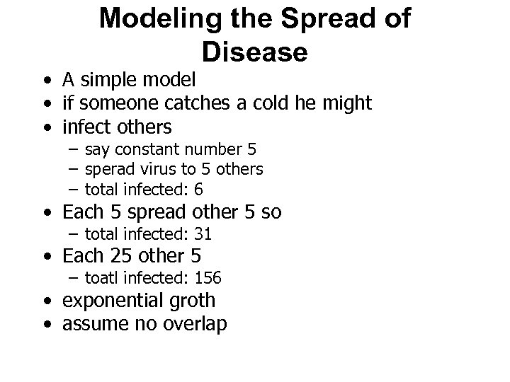
Modeling the Spread of Disease • A simple model • if someone catches a cold he might • infect others – say constant number 5 – sperad virus to 5 others – total infected: 6 • Each 5 spread other 5 so – total infected: 31 • Each 25 other 5 – toatl infected: 156 • exponential groth • assume no overlap
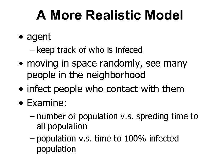
A More Realistic Model • agent – keep track of who is infeced • moving in space randomly, see many people in the neighborhood • infect people who contact with them • Examine: – number of population v. s. spreding time to all population – population v. s. time to 100% infected population
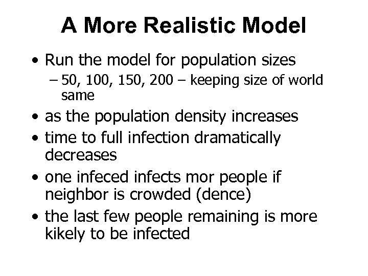
A More Realistic Model • Run the model for population sizes – 50, 100, 150, 200 – keeping size of world same • as the population density increases • time to full infection dramatically decreases • one infeced infects mor people if neighbor is crowded (dence) • the last few people remaining is more kikely to be infected
A More Realistic Model • Runing model several times produces different data • Most ABMs – randomness – the code includes random number generators • E. g. : in So. DM – movemnts of agents at each time step • Table 6. 3 ten runs with the same parameter set
Statistical Analysis of ABM: Moving • Data generated from – natural experiments, – computer programs • • • Descriptive statistics E. g. : hypothesis a coin is fair H 0 p=0. 5 HA P 0. 5 test based on obsered probablity and standard deviation
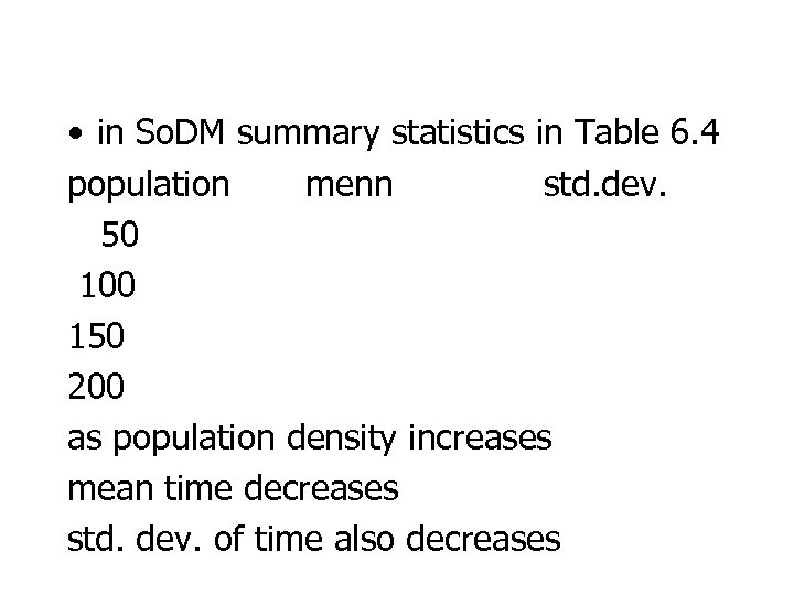
• in So. DM summary statistics in Table 6. 4 population menn std. dev. 50 100 150 200 as population density increases mean time decreases std. dev. of time also decreases
• Develop hypothesis about hwo inputs affects outputs • ABMs produces large amounts of data • Net. Logo Mathematica • Net. Logo R extension
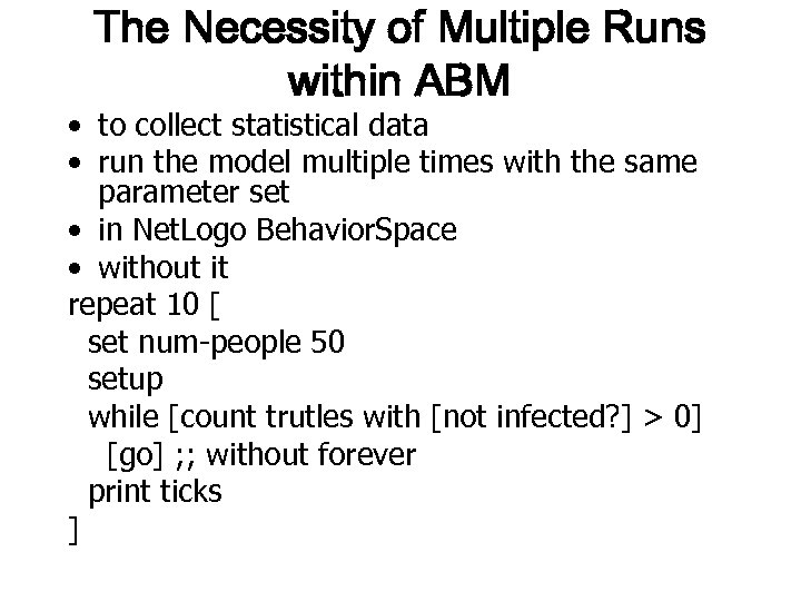
The Necessity of Multiple Runs within ABM • to collect statistical data • run the model multiple times with the same parameter set • in Net. Logo Behavior. Space • without it repeat 10 [ set num-people 50 setup while [count trutles with [not infected? ] > 0] [go] ; ; without forever print ticks ]
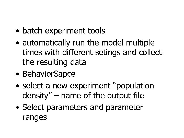
• batch experiment tools • automatically run the model multiple times with different setings and collect the resulting data • Behavior. Sapce • select a new experiment “population density” – name of the output file • Select parameters and parameter ranges
![[“num-people” 50] • sets NUM-PEOPLE to 50 [“num-people” [50 50 200]] • sets NUM-PEOPLE [“num-people” 50] • sets NUM-PEOPLE to 50 [“num-people” [50 50 200]] • sets NUM-PEOPLE](https://present5.com/presentation/843ca9fdf1c48f265c6acd47552a30d7/image-15.jpg)
[“num-people” 50] • sets NUM-PEOPLE to 50 [“num-people” [50 50 200]] • sets NUM-PEOPLE from 50 to 200 incremented by 50 • onther parameter at the same time • NUM-INFECTED [“num-infected” [1 1 5]] • all combinations of the two parameters
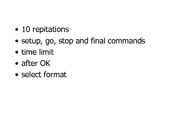
• • • 10 repitations setup, go, stop and final commands time limit after OK select format

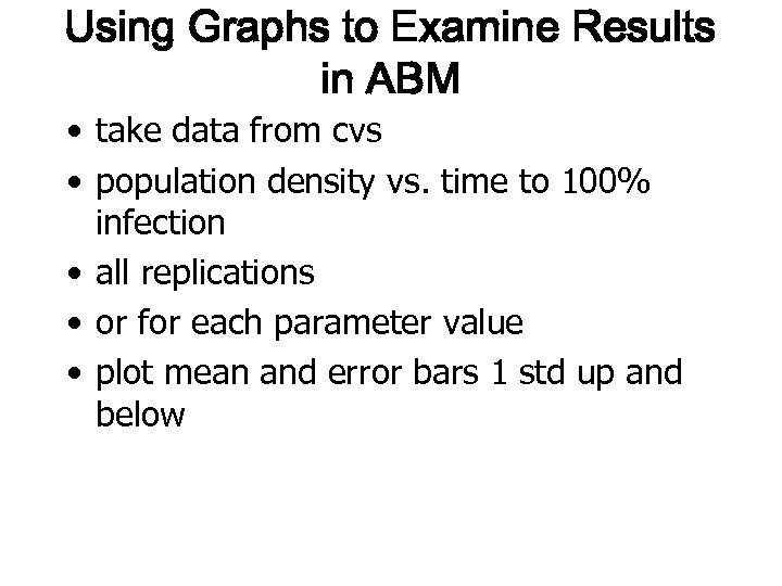
Using Graphs to Examine Results in ABM • take data from cvs • population density vs. time to 100% infection • all replications • or for each parameter value • plot mean and error bars 1 std up and below
Time series graphes • • • values of variables vs. time (ticks) in ABM most dat temporal number-of-people-infected vs. time figure 6. 6 three phases – first phase: slowly increase – few infected – second phase: increases sharply – nany infeced infects otghers – third phase: indectionrate slows again – few people remains uninfected
• multiple graphs in the same figure for different vaues of parameters • or • mean – X*std, mean+X*std • vs. time graphs
Analyzing Networks within ABM • • • many interactions in social networks E. g. : So. DM chooser – “network” Erdos Renyi random graph parameter – connections per node; average degree of the network – how many connections an individual with other individuals on the average • connection per node : 4
Experiments • number of people infeced may not be 200 – not all people are infected • experiment with paramter – connection per node – critical point is around 1. 0 • set time limit to 50 • ANC: from 0. 5 to 4. 0 at incremets of 0. 5
• a general characteristics of RN • as average degree exceeds 1. 0 a gient component forms • In clasical epidemics – ratio of rate of infection to rate of recovery – > 1. 0 – population is infeced or – the desies dies out
Other Parameters • • average path length (APL) as APL spread slower as APL spread faster Cllustering coefficient – how tightly the network is clustered – how nany nodes an egent has links are also links with themselfs • ABM and SNA used together
Environmental Data and ABM • • • in spread of a cold agent to environment or environment to agent interactions in So. DM – environmental interaction effect • set variant to “environmental” • parameter DESEAS-DECAY
Experiments • hold num-population at 200 • vary disease-decay from 0 (original) to 10 • Table 6. 7 • as disease-decay time to 100% infection • both num-population and deseasedecay varied – two dimensional graphs Figure 6. 9
patterns • • policy measures quarantine an area of the world? prevents a disease spreading or track each individual and attapt to cure? • if starts from a certain area • put a ring aroud the area snd gradually srink the ring
patterns • • qualitative and quantitaive patterns lanscape metrics – edge density of yellow trails ratio of the number of edges between two states of the environment – infected and uninfeced patches • edge density low – few shared edges – similar patches are highly clustered
Outline Types of Measurements Modeling the Spread of Disease Summarizing Analysis of ABMs
Summarizing Analysis of ABMs • • Analysing ABMs chalenges number of inputs and outputs high outputs at aggregate or individual levels ability to control model but combinatorial explosion • parameters their values – agent environment global • outputs – end values, dynamics over time • START SIMPLE MODELS
Chalenges • vast number of parameters – validation – real data or experiment with – is the model robust to changes to these parameters • vast number of outputs – lost in data – difficulty of finding patterns – relations between inputs and outputs
Formats of Data • • • Four formats of data statistical graphical network spatial Inputs can be specified based on these formats
843ca9fdf1c48f265c6acd47552a30d7.ppt