Minimal Probing Supporting Expensive Predicates for Top -k

Minimal Probing: Supporting Expensive Predicates for Top -k Queries Kevin C. Chang Seung-won Hwang Univ. of Illinois at Urbana-Champaign

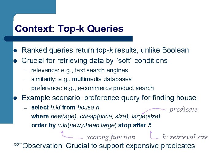
Context: Top-k Queries l l Ranked queries return top-k results, unlike Boolean Crucial for retrieving data by “soft” conditions – – – l relevance: e. g. , text search engines similarity: e. g. , multimedia databases preference: e. g. , e-commerce product search Example scenario: preference query for finding house: – select h. id from house h where new(age), cheap(price, size), large(size) order by min(new, cheap, large) stop after 5 predicate scoring function k: retrieval size FObservation: Crucial to support expensive predicates

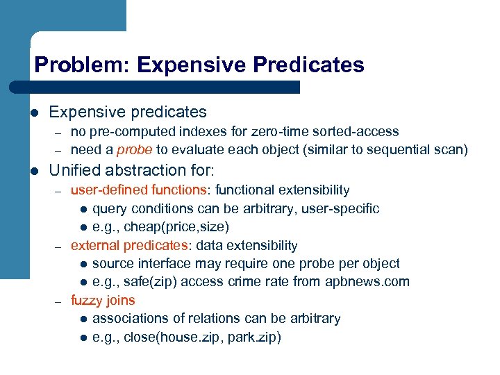
Problem: Expensive Predicates l Expensive predicates – – l no pre-computed indexes for zero-time sorted-access need a probe to evaluate each object (similar to sequential scan) Unified abstraction for: – – – user-defined functions: functional extensibility l query conditions can be arbitrary, user-specific l e. g. , cheap(price, size) external predicates: data extensibility l source interface may require one probe per object l e. g. , safe(zip) access crime rate from apbnews. com fuzzy joins l associations of relations can be arbitrary l e. g. , close(house. zip, park. zip)

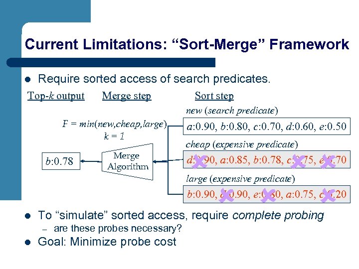
Current Limitations: “Sort-Merge” Framework l Require sorted access of search predicates. Top-k output Merge step Sort step new (search predicate) F = min(new, cheap, large) k=1 b: 0. 78 Merge Algorithm a: 0. 90, b: 0. 80, c: 0. 70, d: 0. 60, e: 0. 50 cheap (expensive predicate) û ûû û d: 0. 90, a: 0. 85, b: 0. 78, c: 0. 75, e: 0. 70 large (expensive predicate) b: 0. 90, d: 0. 90, e: 0. 80, a: 0. 75, c: 0. 20 l To “simulate” sorted access, require complete probing – l are these probes necessary? Goal: Minimize probe cost

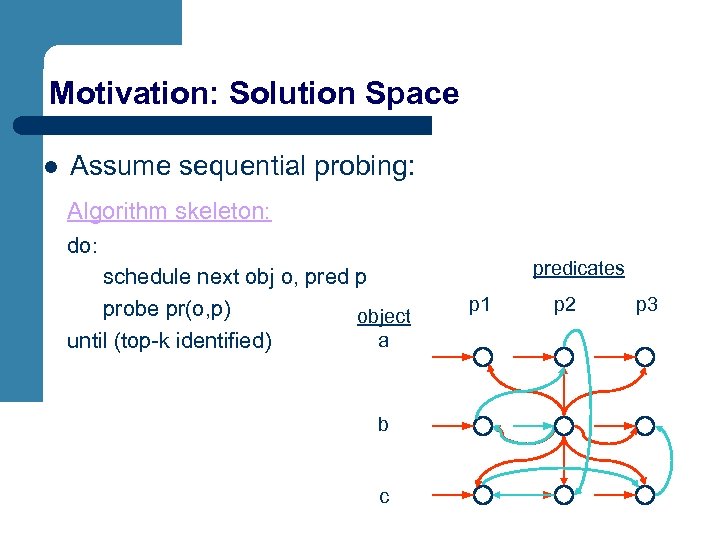
Motivation: Solution Space l Assume sequential probing: Algorithm skeleton: do: schedule next obj o, pred p probe pr(o, p) object a until (top-k identified) b c predicates p 1 p 2 p 3

Our framework: Separate, Global Predicate Scheduling Two important decisions on framework: l Separate predicate scheduling – – l scheduling as separate “optimization” phase before probing avoid run-time scheduling overhead Global predicate scheduling – – – scheduling based on global info (predicate selectivities) lack of per-object information to justify per-object scheduling avoid per-object scheduling overhead FSimple framework and algorithm – – – and efficient! allow essentially A* framework, for given predicate schedule enable formal analysis: optimality, scalability

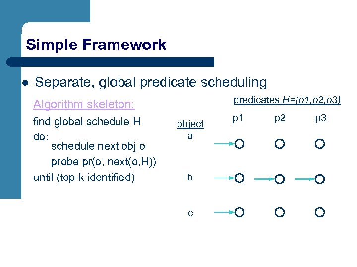
Simple Framework l Separate, global predicate scheduling predicates H=(p 1, p 2, p 3) Algorithm skeleton: find global schedule H do: schedule next obj o probe pr(o, next(o, H)) until (top-k identified) object a b c p 1 p 2 p 3

Challenges for Minimizing Probing l Predicate scheduling before probing – l how to identify the best H? Object scheduling during probing – how to find next object to probe, for achieving “minimal probing” with respect to H? Algorithm skeleton: ? find global schedule H do: schedule next obj o probe pr(o, next(o, H)) until (top-k identified) ?

Challenge 1: Object Scheduling l Goal: Perform only necessary probes l Necessary probes: – A probe is necessary if top-k answers cannot be determined by any algorithm without it, regardless of the outcomes of other probes. FQuestion 1: Given a probe pr(o, next(o, H)), how to determine if it is necessary? l Probe-optimal algorithm – An algorithm is probe-optimal if it performs only the necessary probes. FQuestion 2: How to identify necessary probes in order to design such an algorithm?

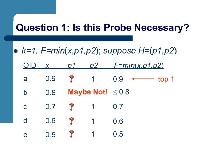
Question 1: Is this Probe Necessary? l k=1, F=min(x, p 1, p 2); suppose H=(p 1, p 2) OID x p 1 p 2 F=min(x, p 1, p 2) a 0. 9 1 ? 1 0. 9 b 0. 8 Maybe Not! £ 0. 8 ? c 0. 7 1 ? 1 0. 7 d 0. 6 1 ? 1 0. 6 e 0. 5 1 ? 1 0. 5 top 1

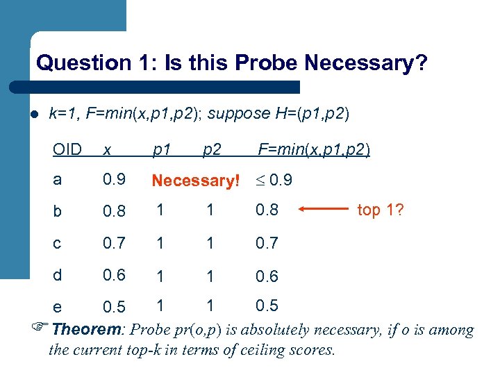
Question 1: Is this Probe Necessary? l k=1, F=min(x, p 1, p 2); suppose H=(p 1, p 2) OID x p 1 p 2 F=min(x, p 1, p 2) a 0. 9 Necessary! £ 0. 9 ? b 0. 8 1 1 0. 8 c 0. 7 1 1 0. 7 d 0. 6 1 1 0. 6 top 1? 1 1 0. 5 e 0. 5 FTheorem: Probe pr(o, p) is absolutely necessary, if o is among the current top-k in terms of ceiling scores.

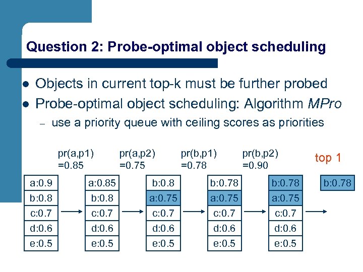
Question 2: Probe-optimal object scheduling l l Objects in current top-k must be further probed Probe-optimal object scheduling: Algorithm MPro – use a priority queue with ceiling scores as priorities pr(a, p 1) =0. 85 pr(a, p 2) =0. 75 pr(b, p 1) =0. 78 pr(b, p 2) =0. 90 a: 0. 9 b: 0. 8 a: 0. 85 b: 0. 8 a: 0. 75 b: 0. 78 a: 0. 75 c: 0. 7 d: 0. 6 e: 0. 5 top 1 b: 0. 78

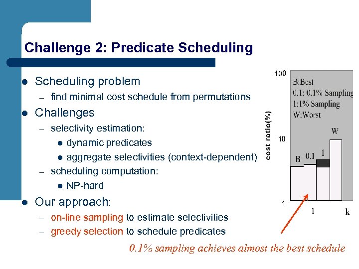
Challenge 2: Predicate Scheduling l Scheduling problem – l Challenges – – l find minimal cost schedule from permutations selectivity estimation: l dynamic predicates l aggregate selectivities (context-dependent) scheduling computation: l NP-hard Our approach: – – on-line sampling to estimate selectivities greedy selection to schedule predicates 0. 1% sampling achieves almost the best schedule

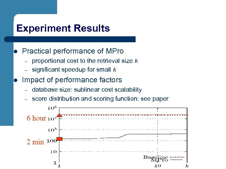
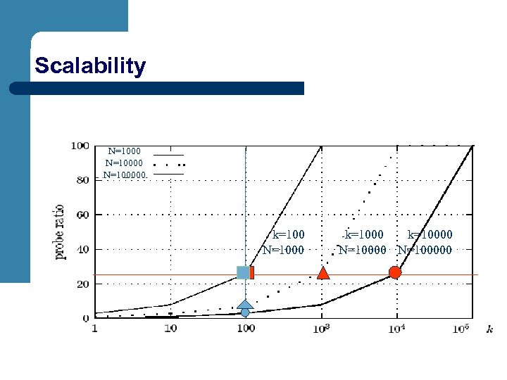
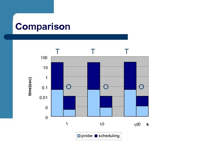
Experiment Results l Practical performance of MPro – – l proportional cost to the retrieval size k significant speedup for small k Impact of performance factors – – database size: sublinear cost scalability score distribution and scoring function: see paper 6 hour 2 min

Demo : House Search l Data: All houses on sale in Illinois (N=20990) – – l from www. realtor. com. objects: house(id, price, size, bed, bath, zip, city) Query: F = Average(n, c, r) – n nearcity: close to Chicago – c cheap: “reasonable” price for its size – r roomy: prefer 4 -6 rooms

Summary of Contributions (more in the paper) l Abstraction: – l for user-defined, external, and fuzzy join predicates Framework and algorithm: – – probe-optimal algorithm MPro – l sampling-based global scheduling extensions of MPro: fuzzy joins, parallel MPro, approximation Principles/Theorems: – – probe-optimality of MPro – l necessary-probe principle analytical scalability of MPro Extensive experiments

Thank You!

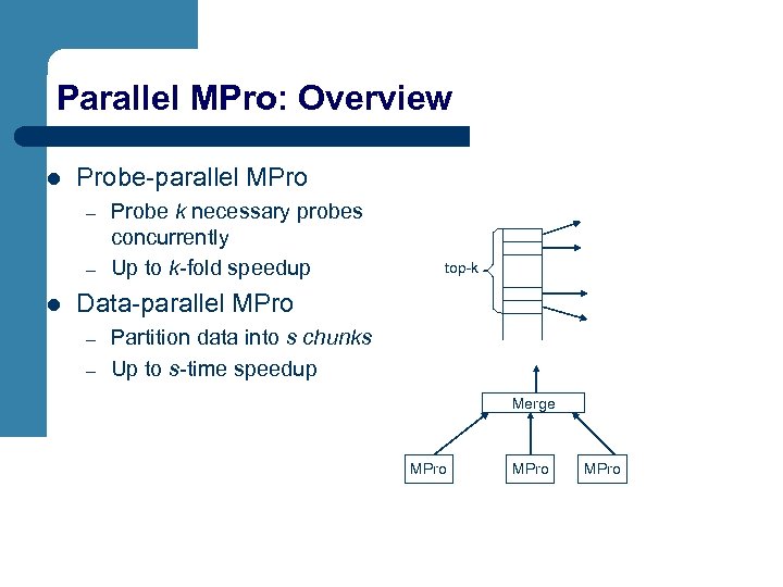
Parallel MPro: Overview l Probe-parallel MPro – – l Probe k necessary probes concurrently Up to k-fold speedup top-k Data-parallel MPro – – Partition data into s chunks Up to s-time speedup Merge MPro

Scalability N=100000 k=100 N=1000 k=10000 N=100000

Comparison T T O O