Midterm 3 Revision and ID 3 Prof Sin-Min

Midterm 3 Revision and ID 3 Prof. Sin-Min Lee

Armstrong’s Axioms • We can find F+ by applying Armstrong’s Axioms: – if , then (reflexivity) – if , then (augmentation) – if , and , then (transitivity) • These rules are – sound (generate only functional dependencies that actually hold) and – complete (generate all functional dependencies that hold).

Additional rules • If and , then (union) • If , then and (decomposition) • If and , then (pseudotransitivity) The above rules can be inferred from Armstrong’s axioms.

Example • R = (A, B, C, G, H, I) F={ A B A C CG H CG I B H} • Some members of F+ – A H • by transitivity from A B and B H – AG I • by augmenting A C with G, to get AG CG and then transitivity with CG I – CG HI • by augmenting CG I to infer CG CGI, and augmenting of CG H to infer CGI HI, and then transitivity

2. Closure of an attribute set • Given a set of attributes A and a set of FDs F, closure of A under F is the set of all attributes implied by A • In other words, the largest B such that: • A B • Redefining super keys: • The closure of a super key is the entire relation schema • Redefining candidate keys: • 1. It is a super key • 2. No subset of it is a super key

Computing the closure for A • Simple algorithm • 1. Start with B = A. • 2. Go over all functional dependencies, , in F+ • 3. If B, then • Add to B • 4. Repeat till B changes

Example • R = (A, B, C, G, H, I) F={ A B A C CG H CG I B H} • (AG) + ? • 1. result = AG 2. result = ABCG (A C and A B) 3. result = ABCGH (CG H and CG AGBC) 4. result = ABCGHI (CG I and CG AGBCH Is (AG) a candidate key ? 1. It is a super key. 2. (A+) = BC, (G+) = G. YES.

Uses of attribute set closures • Determining superkeys and candidate keys • Determining if A B is a valid FD • Check if A+ contains B • Can be used to compute F+

3. Extraneous Attributes • Consider F, and a functional dependency, A B. • “Extraneous”: Are there any attributes in A or B that can be safely removed ? • Without changing the constraints implied by F • • Example: Given F = {A C, AB CD} – C is extraneous in AB CD since AB C can be inferred even after deleting C

4. Canonical Cover • A canonical cover for F is a set of dependencies Fc such that – F logically implies all dependencies in Fc, and – Fc logically implies all dependencies in F, and – No functional dependency in Fc contains an extraneous attribute, and – Each left side of functional dependency in Fc is unique • In some (vague) sense, it is a minimal version of F • Read up algorithms to compute Fc

Loss-less Decompositions • Definition: A decomposition of R into (R 1, R 2) is called lossless if, for all legal instance of r(R): r = R 1 (r ) • R 2 (r ) • In other words, projecting on R 1 and R 2, and joining back, results in the relation you started with • Rule: A decomposition of R into (R 1, R 2) is lossless, iff: • R 1 ∩ R 2 R 1 • in F+. or R 1 ∩ R 2

Dependency-preserving Decompositions • • Is it easy to check if the dependencies in F hold ? Okay as long as the dependencies can be checked in the same table. • Consider R = (A, B, C), and F ={A B, B C} • 1. Decompose into R 1 = (A, B), and R 2 = (A, C) • Lossless ? Yes. • But, makes it hard to check for B C • The data is in multiple tables. • 2. On the other hand, R 1 = (A, B), and R 2 = (B, C), • • • is both lossless and dependency-preserving Really ? What about A C ? If we can check A B, and B C, A C is implied.

Dependency-preserving Decompositions • Definition: • Consider decomposition of R into R 1, …, Rn. • Let Fi be the set of dependencies F + that include only attributes in Ri. • The decomposition is dependency preserving, if (F 1 F 2 … Fn )+ = F +

Example • Suppose we have R(A, B, C) with • FD 1. A B • FD 2. A C • FD 3. B C The decomposition R 1(A, B), R 2(A, C) is lossless but not dependency preservation. The decomposition R 1(A, B), R 2(A, C) and R 3(B, C) is dependency preservation.

BCNF • Given a relation schema R, and a set of functional dependencies F, if every FD, A B, is either: • • 1. Trivial 2. A is a superkey of R • Then, R is in BCNF (Boyce-Codd Normal Form) • Why is BCNF good ?

BCNF • What if the schema is not in BCNF ? • Decompose (split) the schema into two pieces. • Careful: you want the decomposition to be lossless

Achieving BCNF Schemas For all dependencies A B in F+, check if A is a superkey • • • By using attribute closure If not, then • Choose a dependency in F+ that breaks the BCNF rules, say A B • Create R 1 = A B • Create R 2 = A (R – B – A) • Note that: R 1 ∩ R 2 = A and A AB (= R 1), so this is lossless decomposition • Repeat for R 1, and R 2 • By defining F 1+ to be all dependencies in F that contain only attributes in R 1 • Similarly F 2+

Example 1 • • R = (A, B, C) • F = {A B, B C} • Candidate keys = {A} BCNF = No. B C violates. B C • • R 1 = (B, C) • F 1 = {B C} Candidate keys = {B} • BCNF = true • • R 2 = (A, B) • F 2 = {A B} Candidate keys = {A} • BCNF = true

Example 2 -1 • R = (A, B, C, D, E) • F = {A B, BC D} • Candidate keys = {ACE} BCNF = Violated by {A B, BC D} etc… • • From A B and BC D by pseudo-transitivity A B • • R 1 = (A, B) • F 1 = {A B} Candidate keys = {A} • BCNF = true • • R 2 = (A, C, D, E) F 2 = {AC D} Candidate keys = {ACE} BCNF = false (AC D) Dependency preservation ? ? ? AC D We can check: A B (R 1), AC D (R 3), but we lost BC D • R 3 = (A, C, D) So this is not a dependency • F 3 = {AC D} • -preserving decomposition • Candidate keys = {AC} • • BCNF = true • R 4 = (A, C, E) F 4 = {} [[ only trivial ]] Candidate keys = {ACE} • BCNF = true

• Example 2 -2 • R = (A, B, C, D, E) • F = {A B, BC D} • Candidate keys = {ACE} BCNF = Violated by {A B, BC D} etc… BC D • • R 1 = (B, C, D) F 1 = {BC D} Candidate keys = {BC} • BCNF = true Dependency preservation ? ? ? We can check: BC D (R 1), A B (R 3), Dependency-preserving decomposition • • • R 2 = (B, C, A, E) • F 2 = {A B} Candidate keys = {ACE} BCNF = false (A B) A B • • R 3 = (A, B) • F 3 = {A B} Candidate keys = {A} • BCNF = true • • • R 4 = (A, C, E) F 4 = {} [[ only trivial ]] Candidate keys = {ACE} • BCNF = true

Example 3 • • R = (A, B, C, D, E, H) • F = {A BC, E HA} • Candidate keys = {DE} BCNF = Violated by {A BC} etc… A BC • • R 1 = (A, B, C) F 1 = {A BC} Candidate keys = {A} • BCNF = true Dependency preservation ? ? ? We can check: A BC (R 1), E HA (R 3), Dependency-preserving decomposition • • R 2 = (A, D, E, H) F 2 = {E HA} Candidate keys = {DE} BCNF = false (E HA) E HA • • • R 3 = (E, H, A) F 3 = {E HA} Candidate keys = {E} • BCNF = true • • • R 4 = (ED) F 4 = {} [[ only trivial ]] Candidate keys = {DE} • BCNF = true

Classification vs. Prediction • Classification: – When a classifier is build it predicts categorical class labels of new data – classifies unknown data. We also say that it predicts class labels of the new data – Construction of the classifier (a model) is based on a training set in which the values of a decision attribute (class labels) are given and is tested on a test set • Prediction – Statistical method that models continuous-valued functions, i. e. , predicts unknown or missing values

Classification Process : Model Construction Training Data Classification Algorithms Classifier (Model) IF rank = ‘professor’ OR years > 6 THEN tenured = ‘yes’

Testing and Prediction (by a classifier) Classifier Testing Data Unseen Data (Jeff, Professor, 4) Tenured?

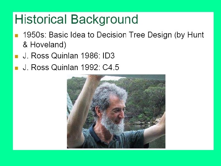
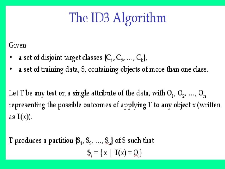
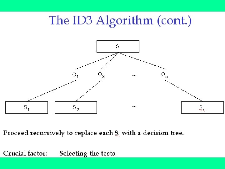
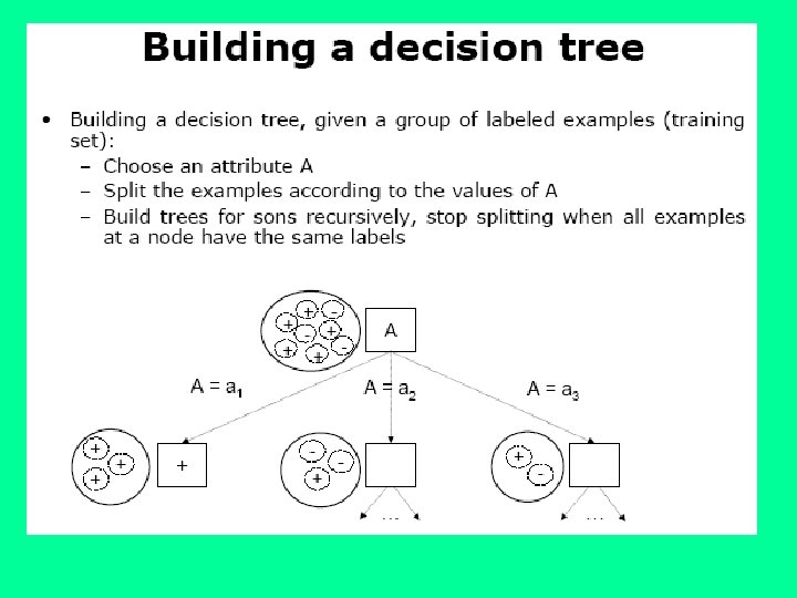
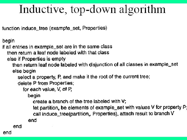
J. Ross Quinlan originally developed ID 3 at the University of Sydney. He first presented ID 3 in 1975 in a book, Machine Learning, vol. 1, no. 1. ID 3 is based off the Concept Learning System (CLS) algorithm. The basic CLS algorithm over a set of training instances C: Step 1: If all instances in C are positive, then create YES node and halt. If all instances in C are negative, create a NO node and halt. Otherwise select a feature, F with values v 1, . . . , vn and create a decision node. Step 2: Partition the training instances in C into subsets C 1, C 2, . . . , Cn according to the values of V. Step 3: apply the algorithm recursively to each of the sets Ci. Note, the trainer (the expert) decides which feature to select.

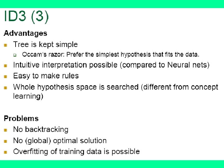
ID 3 improves on CLS by adding a feature selection heuristic. ID 3 searches through the attributes of the training instances and extracts the attribute that best separates the given examples. If the attribute perfectly classifies the training sets then ID 3 stops; otherwise it recursively operates on the n (where n = number of possible values of an attribute) partitioned subsets to get their "best" attribute. The algorithm uses a greedy search, that is, it picks the best attribute and never looks back to reconsider earlier choices.

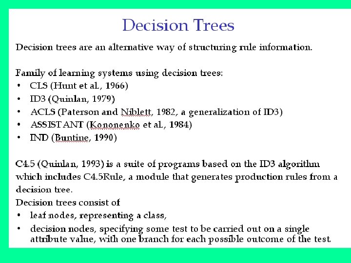
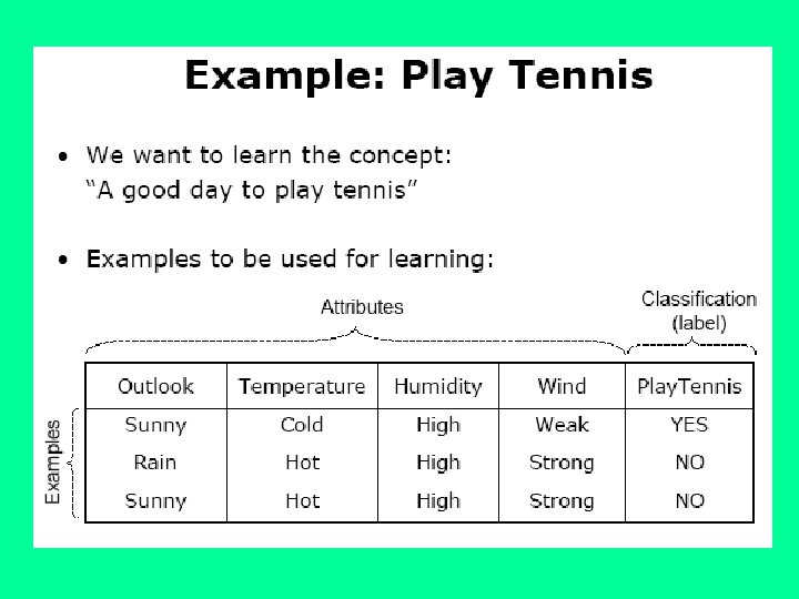
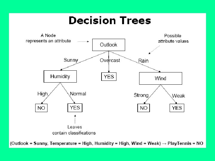
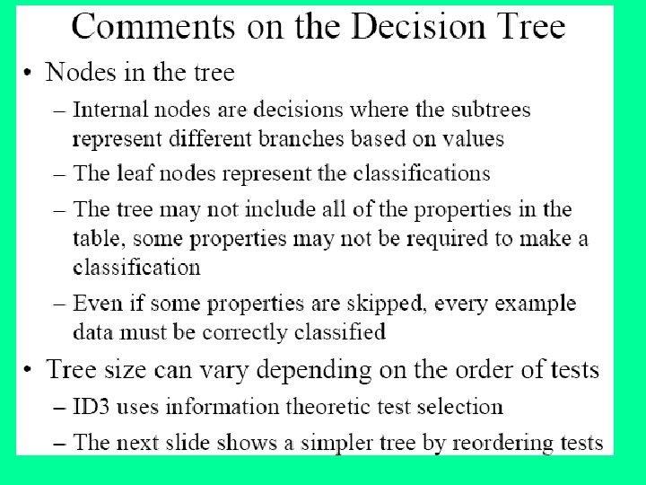
A decision tree is a tree in which each branch node represents a choice between a number of alternatives, and each leaf node represents a classification or decision.

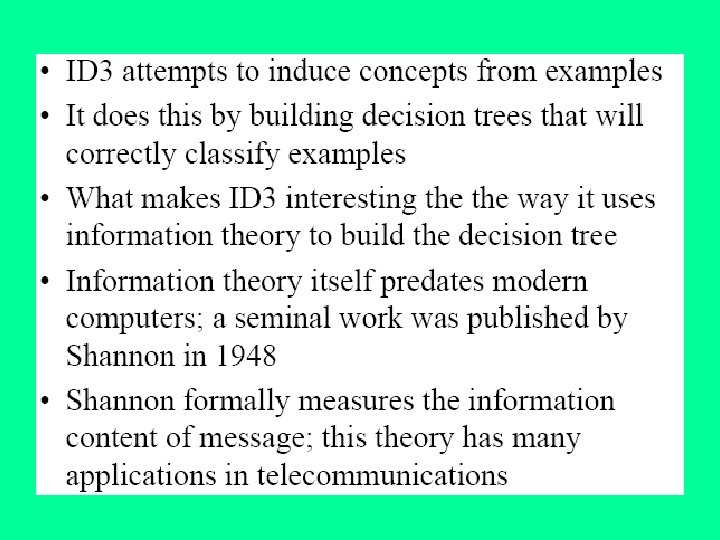
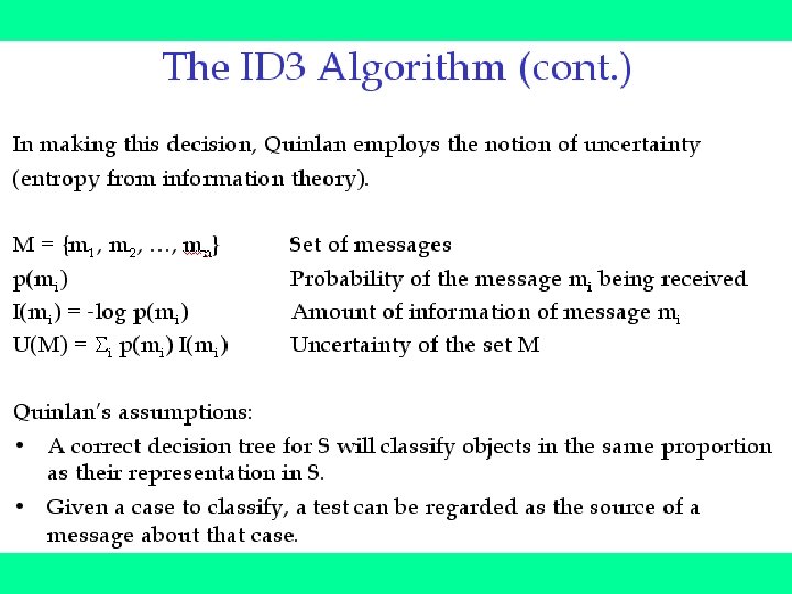
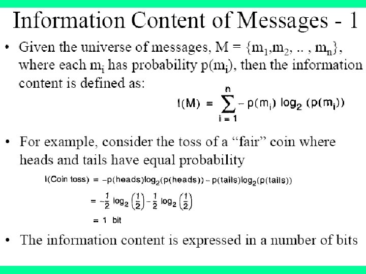
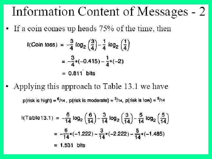
Choosing Attributes and ID 3 • The order in which attributes are chosen determines how complicated the tree is. • ID 3 uses information theory to determine the most informative attribute. • A measure of the information content of a message is the inverse of the probability of receiving the message: • information 1(M) = 1/probability(M) • Taking logs (base 2) makes information correspond to the number of bits required to encode a message: • information(M) = -log 2(probability(M))

Information • The information content of a message should be related to the degree of surprise in receiving the message. • Messages with a high probability of arrival are not as informative as messages with low probability. • Learning aims to predict accurately, i. e. reduce surprise. • Probabilities are multiplied to get the probability of two or more things both/all happening. Taking logarithms of the probabilities allows information to be added instead of multiplied.

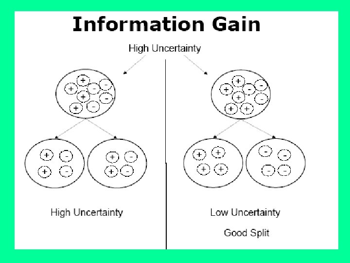
A measure used from Information Theory in the ID 3 algorithm and many others used in decision tree construction is that of Entropy. Informally, the entropy of a dataset can be considered to be how disordered it is. It has been shown that entropy is related to information, in the sense that the higher the entropy, or uncertainty, of some data, then the more information is required in order to completely describe that data. In building a decision tree, we aim to decrease the entropy of the dataset until we reach leaf nodes at which point the subset that we are left with is pure, or has zero entropy and represents instances all of one class (all instances have the same value for the target attribute).

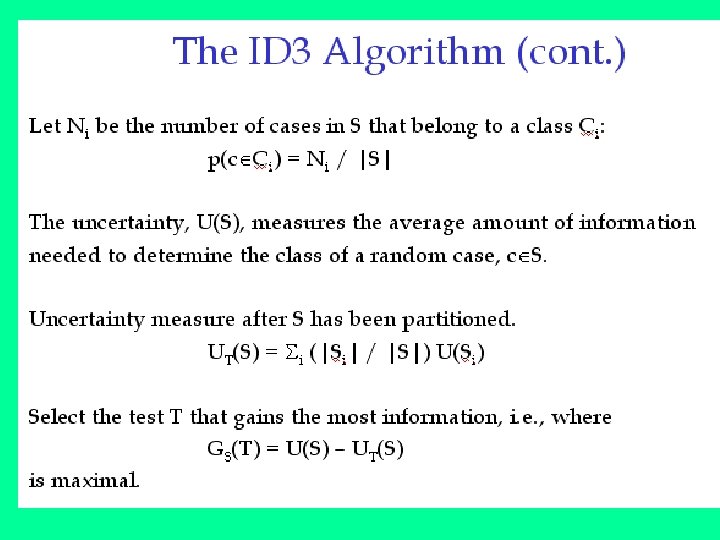
We measure the entropy of a dataset, S, with respect to one attribute, in this case the target attribute, with the following calculation: where Pi is the proportion of instances in the dataset that take the ith value of the target attribute This probability measures give us an indication of how uncertain we are about the data. And we use a log 2 measure as this represents how many bits we would need to use in order to specify what the class (value of the target attribute) is of a random instance.

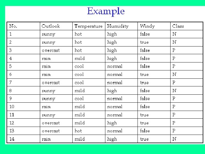
Using the example of the marketing data, we know that there are two classes in the data and so we use the fractions that each class represents in an entropy calculation: Entropy (S = [9/14 responses, 5/14 no responses]) = -9/14 log 2 9/14 - 5/14 log 2 5/14 = 0. 947 bits

Entropy • Different messages have different probabilities of arrival. • Overall level of uncertainty (termed entropy) is: • -Σ P log 2 P • Frequency can be used as a probability estimate. • E. g. if there are 5 +ve examples and 3 -ve examples in a node the estimated probability of +ve is 5/8 = 0. 625.

• Initial decision tree is one node with all examples. • There are 4 +ve examples and 3 -ve examples • i. e. probability of +ve is 4/7 = 0. 57; probability of -ve is 3/7 = 0. 43 • Entropy is: - (0. 57 * log 0. 57) - (0. 43 * log 0. 43) = 0. 99

• Evaluate possible ways of splitting. • Try split on size which has three values: large, medium and small. • There are four instances with size = large. • There are two large positives examples and two large negative examples. • The probability of +ve is 0. 5 • The entropy is: - (0. 5 * log 0. 5) =1

• There is one small +ve and one small -ve • Entropy is: - (0. 5 * log 0. 5) = 1 • There is only one medium +ve and no medium ves, so entropy is 0. • Expected information for a split on size is: • The expected information gain is: 0. 99 - 0. 86 = 0. 13

• Now try splitting on colour and shape. • Colour has an information gain of 0. 52 • Shape has an information gain of 0. 7 • Therefore split on shape. • Repeat for all subtree

Decision Tree for Play. Tennis Outlook Sunny Humidity High No Overcast Rain Yes Normal Yes Wind Strong No Weak Yes

Decision Tree for Play. Tennis Outlook Sunny Humidity High No Overcast Rain Each internal node tests an attribute Normal Yes Each branch corresponds to an attribute value node Each leaf node assigns a classification

Decision Tree for Play. Tennis Outlook Temperature Humidity Wind Play. Tennis Sunny Hot High Weak ? No Outlook Sunny Humidity High No Overcast Rain Yes Normal Yes Wind Strong No Weak Yes

Decision Tree for Conjunction Outlook=Sunny Wind=Weak Outlook Sunny Wind Strong No Overcast No Weak Yes Rain No

Decision Tree for Disjunction Outlook=Sunny Wind=Weak Outlook Sunny Yes Overcast Rain Wind Strong No Wind Weak Yes Strong No Weak Yes

Decision Tree for XOR Outlook=Sunny XOR Wind=Weak Outlook Sunny Wind Strong Yes Overcast Rain Wind Weak No Strong No Wind Weak Yes Strong No Weak Yes

Decision Tree • decision trees represent disjunctions of conjunctions Outlook Sunny Humidity High No Overcast Rain Yes Normal Yes Wind Strong No (Outlook=Sunny Humidity=Normal) (Outlook=Overcast) (Outlook=Rain Wind=Weak) Weak Yes

Information Gain Computation (ID 3/C 4. 5): Case of Two Classes

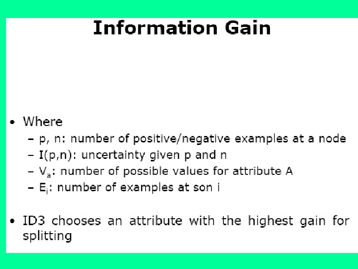
ID 3 algorithm • To get the fastest decision-making procedure, one has to arrange attributes in a decision tree in a proper order - the most discriminating attributes first. This is done by the algorithm called ID 3. • The most discriminating attribute can be defined in precise terms as the attribute for which the fixing its value changes the enthropy of possible decisions at most. Let wj be the frequency of the j-th decision in a set of examples x. Then the enthropy of the set is E(x)= - Swj* log(wj) • Let fix(x, a, v) denote the set of these elements of x whose value of attribute a is v. The average enthropy that remains in x , after the value a has been fixed, is: H(x, a) = S kv E(fix(x, a, v)), where kv is the ratio of examples in x with attribute a having

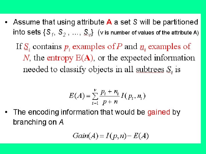
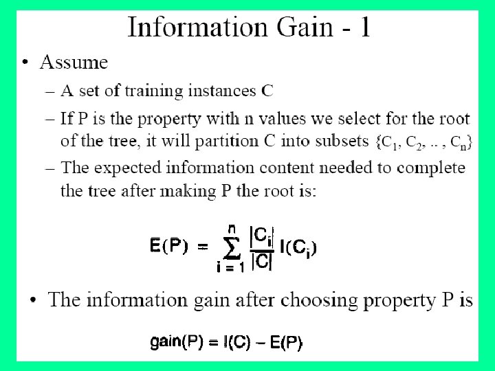
Ok now we want a quantitative way of seeing the effect of splitting the dataset by using a particular attribute (which is part of the tree building process). We can use a measure called Information Gain, which calculates the reduction in entropy (Gain in information) that would result on splitting the data on an attribute, A. where v is a value of A , |Sv| is the subset of instances of S where A takes the value v, and |S| is the number of instances

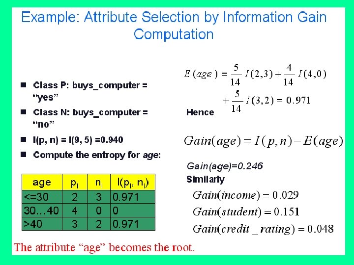
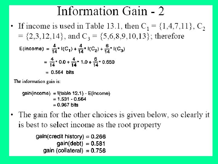
Continuing with our example dataset, let's name it S just for convenience, let's work out the Information Gain that splitting on the attribute District would result in over the entire dataset: So by calculating this value for each attribute that remains, we can see which attribute splits the data more purely. Let's imagine we want to select an attribute for the root node, then performing the above calcualtion for all attributes gives: • Gain(S, House Type) = 0. 049 bits • Gain(S, Income) =0. 151 bits • Gain(S, Previous Customer) = 0. 048 bits

We can clearly see that District results in the highest reduction in entropy or the highest information gain. We would therefore choose this at the root node splitting the data up into subsets corresponding to all the different values for the District attribute. With this node evaluation technique we can procede recursively through the subsets we create until leaf nodes have been reached throughout and all subsets are pure with zero entropy. This is exactly how ID 3 and other variants work.

Example 1 If S is a collection of 14 examples with 9 YES and 5 NO examples then Entropy(S) = - (9/14) Log 2 (9/14) - (5/14) Log 2 (5/14) = 0. 940 Notice entropy is 0 if all members of S belong to the same class (the data is perfectly classified). The range of entropy is 0 ("perfectly classified") to 1 ("totally random"). Gain(S, A) is information gain of example set S on attribute A is defined as Gain(S, A) = Entropy(S) - S ((|Sv| / |S|) * Entropy(Sv)) Where: S is each value v of all possible values of attribute A Sv = subset of S for which attribute A has value v |Sv| = number of elements in Sv |S| = number of elements in S

Example 2. Suppose S is a set of 14 examples in which one of the attributes is wind speed. The values of Wind can be Weak or Strong. The classification of these 14 examples are 9 YES and 5 NO. For attribute Wind, suppose there are 8 occurrences of Wind = Weak and 6 occurrences of Wind = Strong. For Wind = Weak, 6 of the examples are YES and 2 are NO. For Wind = Strong, 3 are YES and 3 are NO. Therefore Gain(S, Wind)=Entropy(S)-(8/14)*Entropy(Sweak)(6/14)*Entropy(Sstrong) = 0. 940 - (8/14)*0. 811 - (6/14)*1. 00 = 0. 048 Entropy(Sweak) = - (6/8)*log 2(6/8) - (2/8)*log 2(2/8) = 0. 811 Entropy(Sstrong) = - (3/6)*log 2(3/6) = 1. 00 For each attribute, the gain is calculated and the highest gain is used in the decision node.

Decision Tree Construction Algorithm (pseudo-code): Input: A data set, S Output: A decision tree • If all the instances have the same value for the target attribute then return a decision tree that is simply this value (not really a tree - more of a stump). • Else 1. Compute Gain values (see above) for all attributes and select an attribute with the lowest value and create a node for that attribute. 2. Make a branch from this node for every value of the attribute 3. Assign all possible values of the attribute to branches. 4. Follow each branch by partitioning the dataset to be only instances whereby the value of the branch is present and then go back to 1.

See the following articles for detail ID 3 algorithm: (1)http: //www. dcs. napier. ac. uk/~peter/vldb/dm/node 11. html (2)http: //www. cse. unsw. edu. au/~billw/cs 9414/notes/ml/06 prop/ id 3/id 3. html