00f3b11f3526b145763d4d0497399c5f.ppt
- Количество слайдов: 40

MBA (Trimester) Module Title : Project Finance and Management Term V UNIT II: – Project Market and Demand Analysis
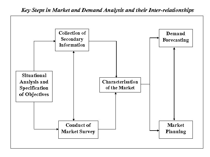
Key Steps in Market and Demand Analysis and their Inter-relationships Collection of Secondary Information Situational Analysis and Specification of Objectives Demand Forecasting Characterisation of the Market Conduct of Market Survey Market Planning
Situational Analysis In order to get a “feel” of the relationship between the product and its market, the project analyst may informally talk to customers, competitors, middlemen, and others in the industry. Wherever possible, he may look at the experience of the company to learn about the preferences and purchasing power of customers, actions and strategies of competitors, and practices of the middlemen.
Collection of Secondary Information n Secondary information is information that has been gathered in some other context and is readily available. n Secondary information provides the base and the starting point for the market and demand analysis. It indicates what is known and often provides leads and cues for gathering primary information required for further analysis.
Evaluation of Secondary Information While secondary information is available economically and readily (provided the market analyst is able to locate it), its reliability, accuracy, and relevance for the purpose under consideration must be carefully examined. The market analyst should seek to know: Who gathered the information? What was the objective? When was the information gathered? When was it published? How representative was the period for which the information was gathered? Have the terms in the study been carefully and unambiguously defined? What was the target population? How was the sample chosen? How representative was the sample? How satisfactory was the process of information gathering? What was the degree of sampling bias and non-response bias in the information gathered? What was the degree of misrepresentation by respondents?
Market Survey n Secondary information, though useful, often does not provide a comprehensive basis for market and demand analysis. It needs to be supplemented with primary information gathered through a market survey. n The market survey may be a census survey or a sample survey; typically it is the latter.
Information Sought in a Market Survey The information sought in a market survey may relate to one or more of the following: Total demand rate of growth of demand Demand in different segments of the market Income and price elasticities of demand Motives for buying Purchasing plans and intentions Satisfaction with existing products Unsatisfied needs Attitudes toward various products Distributive trade practices and preferences Socio-economic characteristics of buyers
Steps in a Sample Survey Typically, a sample survey involves the following steps: 1. Define the target population. 2. Select the sampling scheme and sample size. 3. Develop the questionnaire. 4. Recruit and train the field investigators. 5. Obtain information as per the questionnaire from the sample of respondents. 6. Scrutinise the information gathered. 7. Analyse and interpret the information.
Characterisation of the Market Based on the information gathered from secondary sources and through the market survey, the market for the product/service may be described in terms of the following: • Effective demand in the past and present • Breakdown of demand • Price • Methods of distribution and sales promotion • Consumers • Supply and competition • Government policy
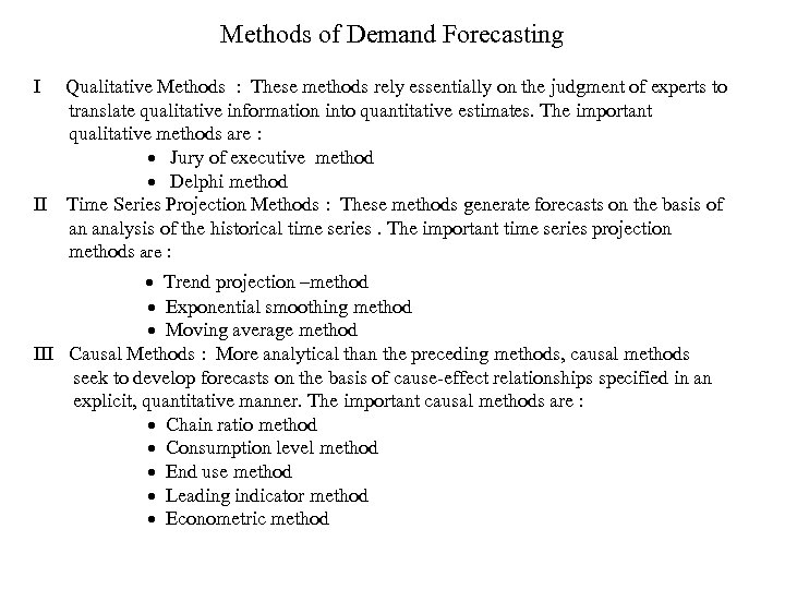
Methods of Demand Forecasting I Qualitative Methods : These methods rely essentially on the judgment of experts to translate qualitative information into quantitative estimates. The important qualitative methods are : Jury of executive method Delphi method II Time Series Projection Methods : These methods generate forecasts on the basis of an analysis of the historical time series. The important time series projection methods are : Trend projection –method Exponential smoothing method Moving average method III Causal Methods : More analytical than the preceding methods, causal methods seek to develop forecasts on the basis of cause-effect relationships specified in an explicit, quantitative manner. The important causal methods are : Chain ratio method Consumption level method End use method Leading indicator method Econometric method
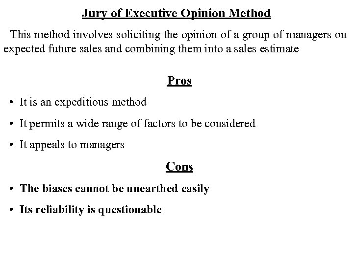
Jury of Executive Opinion Method This method involves soliciting the opinion of a group of managers on expected future sales and combining them into a sales estimate Pros • It is an expeditious method • It permits a wide range of factors to be considered • It appeals to managers Cons • The biases cannot be unearthed easily • Its reliability is questionable
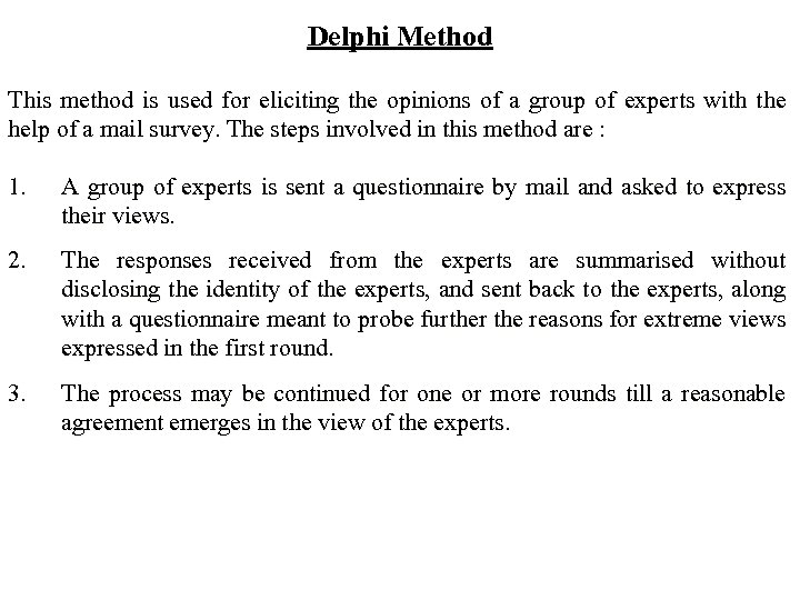
Delphi Method This method is used for eliciting the opinions of a group of experts with the help of a mail survey. The steps involved in this method are : 1. A group of experts is sent a questionnaire by mail and asked to express their views. 2. The responses received from the experts are summarised without disclosing the identity of the experts, and sent back to the experts, along with a questionnaire meant to probe further the reasons for extreme views expressed in the first round. 3. The process may be continued for one or more rounds till a reasonable agreement emerges in the view of the experts.
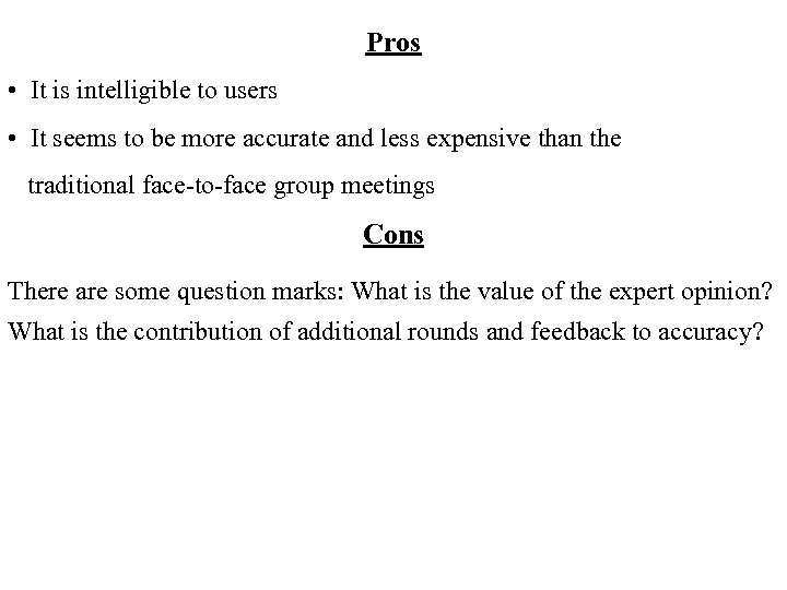
Pros • It is intelligible to users • It seems to be more accurate and less expensive than the traditional face-to-face group meetings Cons There are some question marks: What is the value of the expert opinion? What is the contribution of additional rounds and feedback to accuracy?
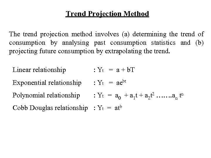
Trend Projection Method The trend projection method involves (a) determining the trend of consumption by analysing past consumption statistics and (b) projecting future consumption by extrapolating the trend. Linear relationship : Yt = a + b. T Exponential relationship : Yt = aebt Polynomial relationship : Yt = a 0 + a 1 t + a 2 t 2 ……. an tn Cobb Douglas relationship : Yt = atb
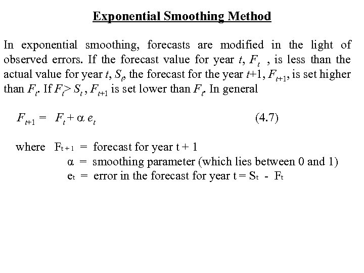
Exponential Smoothing Method In exponential smoothing, forecasts are modified in the light of observed errors. If the forecast value for year t, Ft , is less than the actual value for year t, St, the forecast for the year t+1, Ft+1, is set higher than Ft. If Ft> St , Ft+1 is set lower than Ft. In general Ft+1 = Ft + a et (4. 7) where Ft + 1 = forecast for year t + 1 α = smoothing parameter (which lies between 0 and 1) et = error in the forecast for year t = St - Ft
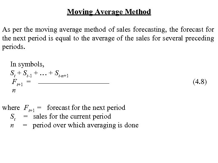
Moving Average Method As per the moving average method of sales forecasting, the forecast for the next period is equal to the average of the sales for several preceding periods. In symbols, St + St-1 + … + St-n+1 Ft+1 = n where Ft+1 = forecast for the next period St = sales for the current period n = period over which averaging is done (4. 8)
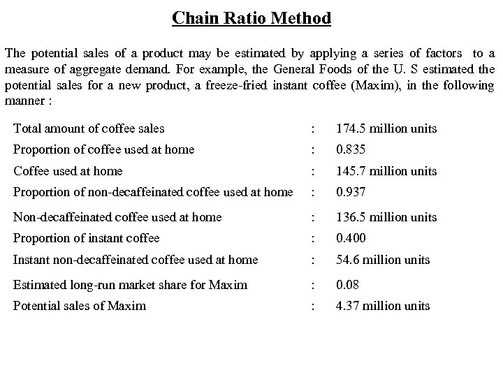
Chain Ratio Method The potential sales of a product may be estimated by applying a series of factors to a measure of aggregate demand. For example, the General Foods of the U. S estimated the potential sales for a new product, a freeze-fried instant coffee (Maxim), in the following manner : Total amount of coffee sales : 174. 5 million units Proportion of coffee used at home : 0. 835 Coffee used at home : 145. 7 million units Proportion of non-decaffeinated coffee used at home : 0. 937 Non-decaffeinated coffee used at home : 136. 5 million units Proportion of instant coffee : 0. 400 Instant non-decaffeinated coffee used at home : 54. 6 million units Estimated long-run market share for Maxim : 0. 08 Potential sales of Maxim : 4. 37 million units
Consumption Level Method The method estimates consumption level on the basis of elasticity coefficients, the important ones being the income elasticity of demand the price elasticity of demand.
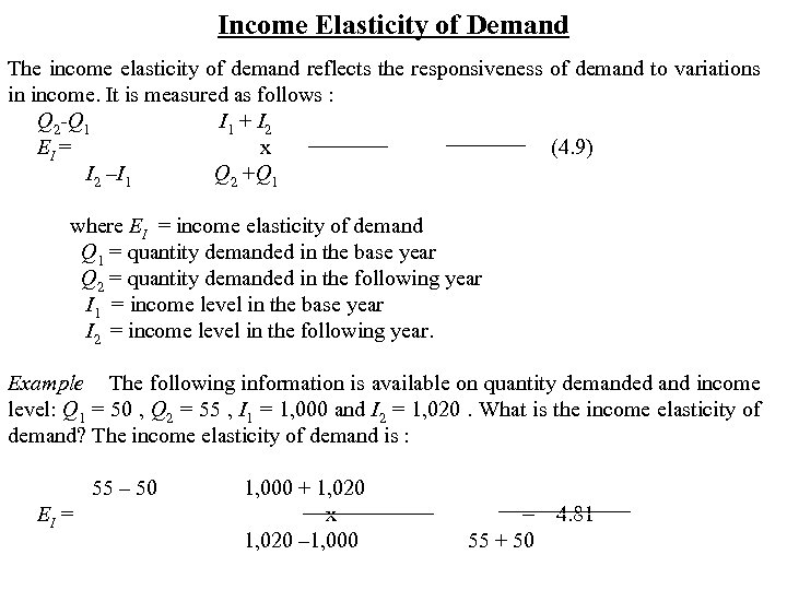
Income Elasticity of Demand The income elasticity of demand reflects the responsiveness of demand to variations in income. It is measured as follows : Q 2 -Q 1 I 1 + I 2 EI = x (4. 9) I 2 –I 1 Q 2 +Q 1 where EI = income elasticity of demand Q 1 = quantity demanded in the base year Q 2 = quantity demanded in the following year I 1 = income level in the base year I 2 = income level in the following year. Example The following information is available on quantity demanded and income level: Q 1 = 50 , Q 2 = 55 , I 1 = 1, 000 and I 2 = 1, 020. What is the income elasticity of demand? The income elasticity of demand is : 55 – 50 1, 000 + 1, 020 EI = x = 4. 81 1, 020 – 1, 000 55 + 50
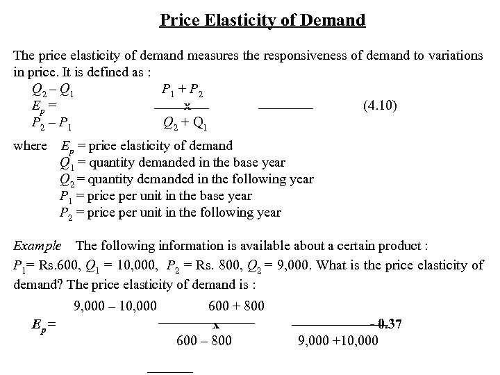
Price Elasticity of Demand The price elasticity of demand measures the responsiveness of demand to variations in price. It is defined as : Q 2 – Q 1 P 1 + P 2 Ep = x (4. 10) P 2 – P 1 Q 2 + Q 1 where Ep = price elasticity of demand Q 1 = quantity demanded in the base year Q 2 = quantity demanded in the following year P 1 = price per unit in the base year P 2 = price per unit in the following year Example The following information is available about a certain product : P 1= Rs. 600, Q 1 = 10, 000, P 2 = Rs. 800, Q 2 = 9, 000. What is the price elasticity of demand? The price elasticity of demand is : 9, 000 – 10, 000 600 + 800 Ep = x = - 0. 37 600 – 800 9, 000 +10, 000
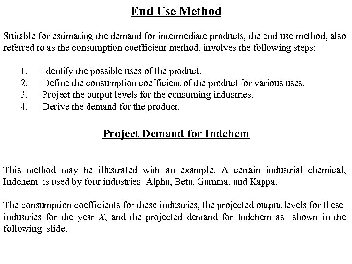
End Use Method Suitable for estimating the demand for intermediate products, the end use method, also referred to as the consumption coefficient method, involves the following steps: 1. Identify the possible uses of the product. 2. Define the consumption coefficient of the product for various uses. 3. Project the output levels for the consuming industries. 4. Derive the demand for the product. Project Demand for Indchem This method may be illustrated with an example. A certain industrial chemical, Indchem is used by four industries Alpha, Beta, Gamma, and Kappa. The consumption coefficients for these industries, the projected output levels for these industries for the year X, and the projected demand for Indchem as shown in the following slide.
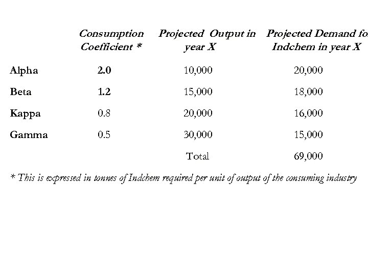
Consumption Coefficient * Projected Output in Projected Demand for year X Indchem in year X Alpha 2. 0 10, 000 20, 000 Beta 1. 2 15, 000 18, 000 Kappa 0. 8 20, 000 16, 000 Gamma 0. 5 30, 000 15, 000 Total 69, 000 * This is expressed in tonnes of Indchem required per unit of output of the consuming industry
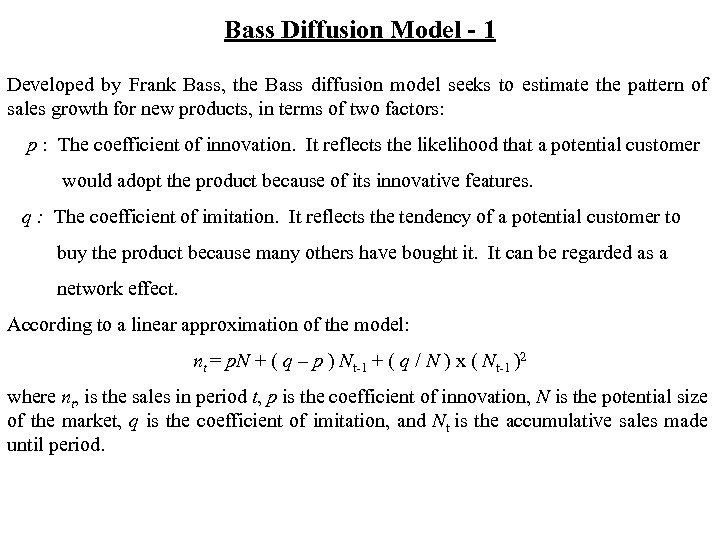
Bass Diffusion Model - 1 Developed by Frank Bass, the Bass diffusion model seeks to estimate the pattern of sales growth for new products, in terms of two factors: p : The coefficient of innovation. It reflects the likelihood that a potential customer would adopt the product because of its innovative features. q : The coefficient of imitation. It reflects the tendency of a potential customer to buy the product because many others have bought it. It can be regarded as a network effect. According to a linear approximation of the model: nt = p. N + ( q – p ) Nt-1 + ( q / N ) x ( Nt-1 )2 where nt, is the sales in period t, p is the coefficient of innovation, N is the potential size of the market, q is the coefficient of imitation, and Nt is the accumulative sales made until period.
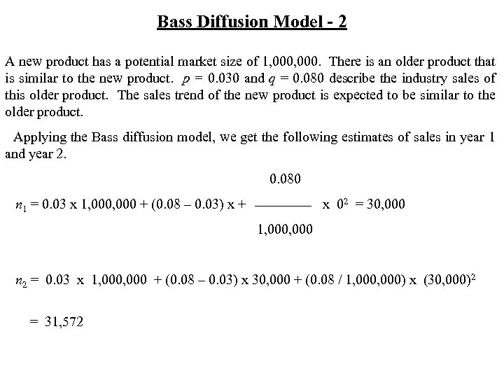
Bass Diffusion Model - 2 A new product has a potential market size of 1, 000. There is an older product that is similar to the new product. p = 0. 030 and q = 0. 080 describe the industry sales of this older product. The sales trend of the new product is expected to be similar to the older product. Applying the Bass diffusion model, we get the following estimates of sales in year 1 and year 2. 0. 080 n 1 = 0. 03 x 1, 000 + (0. 08 – 0. 03) x + x 02 = 30, 000 1, 000 n 2 = 0. 03 x 1, 000 + (0. 08 – 0. 03) x 30, 000 + (0. 08 / 1, 000) x (30, 000)2 = 31, 572
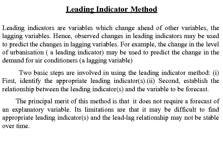
Leading Indicator Method Leading indicators are variables which change ahead of other variables, the lagging variables. Hence, observed changes in leading indicators may be used to predict the changes in lagging variables. For example, the change in the level of urbanisation ( a leading indicator) may be used to predict the change in the demand for air conditioners (a lagging variable) Two basic steps are involved in using the leading indicator method: (i) First, identify the appropriate leading indicator(s). (ii) Second, establish the relationship between the leading indicator(s) and the variable to be forecast. The principal merit of this method is that it does not require a forecast of an explanatory variable. Its limitations are that it may be difficult to find appropriate leading indicator(s) and the lead-lag relationship may not be stable over time.
Econometric Method n An econometric model is a mathematical representation of economic relationship(s) derived from economic theory. The primary objective of econometric analysis is to forecast the future behaviour of the economic variables incorporated in the model. n Two types of econometric models are employed: the single equation model and the simultaneous equation model
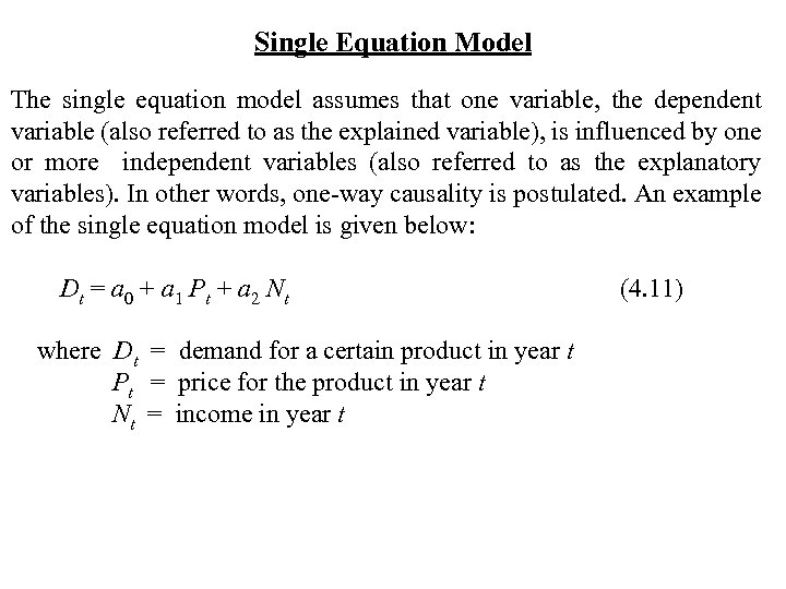
Single Equation Model The single equation model assumes that one variable, the dependent variable (also referred to as the explained variable), is influenced by one or more independent variables (also referred to as the explanatory variables). In other words, one-way causality is postulated. An example of the single equation model is given below: Dt = a 0 + a 1 Pt + a 2 Nt (4. 11) where Dt = demand for a certain product in year t Pt = price for the product in year t Nt = income in year t
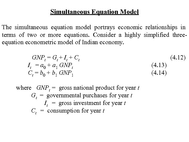
Simultaneous Equation Model The simultaneous equation model portrays economic relationships in terms of two or more equations. Consider a highly simplified threeequation econometric model of Indian economy. GNPt = Gt + It + Ct (4. 12) It = a 0 + a 1 GNPt (4. 13) Ct = b 0 + b 1 GNP 1 (4. 14) where GNPt = gross national product for year t Gt = governmental purchases for year t It = gross investment for year t Ct = consumption for year t
Improving Forecasts You can improve forecasts by following some simple guidelines: • Check assumptions • Stress fundamentals • Beware of history • Watch out for euphoria • Don’t be dazzled by technology • Stay flexible
Uncertainties in Demand Forecasting Demand forecasts are subject to error and uncertainty which arise from three principal sources: • Data about past and present market • Methods of forecasting • Environmental change
Coping with Uncertainties Given the uncertainties in demand forecasting, adequate efforts, along the following lines, may be made to cope with uncertainties. n Conduct analysis with data based on uniform and standard definitions. n In identifying trends, coefficients, and relationships, ignore the abnormal or out-of- the- ordinary observations. n Critically evaluate the assumptions of the forecasting methods and choose a method which is appropriate to the situation. n Adjust the projections derived from quantitative analysis in the light of unquantifiable, but significant, influences. n Monitor the environment imaginatively to identify important changes. n Consider likely alternative scenarios and their impact on market and competition. n Conduct sensitivity analysis to assess the impact on the size of demand for unfavourable and favourable variations of the determining factors from their most likely levels.
Market Planning A marketing plan usually has the following components: • Current marketing situation • Opportunity and issue analysis • Objectives • Marketing strategy • Action programme
SUMMARY n Given the importance of market and demand analysis, it should be carried out in an orderly and systematic manner. The key steps in such analysis are (i) situational analysis and specification of objectives, (ii) collection of secondary information, (iii) conduct of market survey, (iv) characterisation of the market, (v) demand forecasting and (vi) market planning. n The project analyst may do an informal situational analysis which in turn may provide the basis for a formal study. n For purposes of market study, information may be obtained from secondary and /or primary sources. n Secondary information is information that has been gathered in some other context and is already available. While secondary information is available economically, its reliability, accuracy, and relevance for the purpose under consideration must be carefully examined. n Secondary information, though useful, often does not provide a comprehensive basis for market and demand analysis. It needs to be supplemented with primary information gathered through a market survey, specific to the project being appraised, that is likely to be a sample survey.
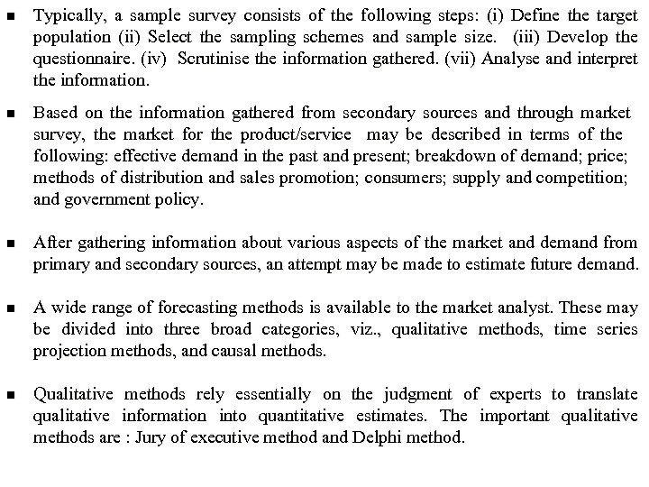
n Typically, a sample survey consists of the following steps: (i) Define the target population (ii) Select the sampling schemes and sample size. (iii) Develop the questionnaire. (iv) Scrutinise the information gathered. (vii) Analyse and interpret the information. n Based on the information gathered from secondary sources and through market survey, the market for the product/service may be described in terms of the following: effective demand in the past and present; breakdown of demand; price; methods of distribution and sales promotion; consumers; supply and competition; and government policy. n After gathering information about various aspects of the market and demand from primary and secondary sources, an attempt may be made to estimate future demand. n A wide range of forecasting methods is available to the market analyst. These may be divided into three broad categories, viz. , qualitative methods, time series projection methods, and causal methods. n Qualitative methods rely essentially on the judgment of experts to translate qualitative information into quantitative estimates. The important qualitative methods are : Jury of executive method and Delphi method.
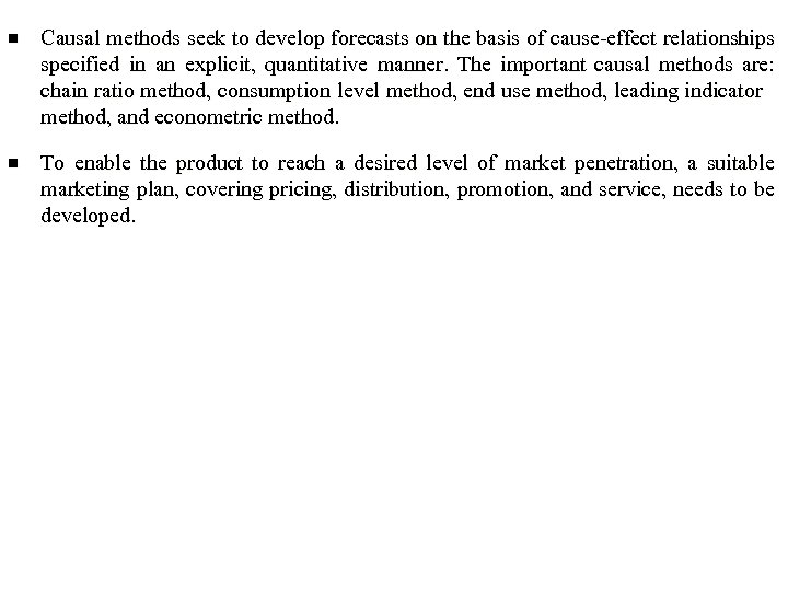
n Causal methods seek to develop forecasts on the basis of cause-effect relationships specified in an explicit, quantitative manner. The important causal methods are: chain ratio method, consumption level method, end use method, leading indicator method, and econometric method. n To enable the product to reach a desired level of market penetration, a suitable marketing plan, covering pricing, distribution, promotion, and service, needs to be developed.
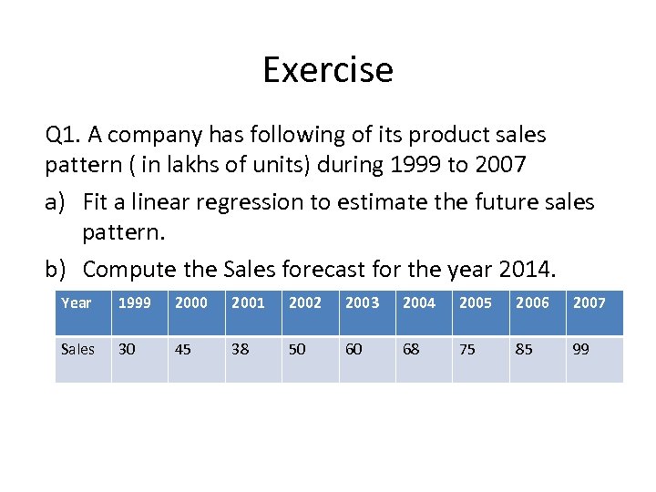
Exercise Q 1. A company has following of its product sales pattern ( in lakhs of units) during 1999 to 2007 a) Fit a linear regression to estimate the future sales pattern. b) Compute the Sales forecast for the year 2014. Year 1999 2000 2001 2002 2003 2004 2005 2006 2007 Sales 30 45 38 50 60 68 75 85 99
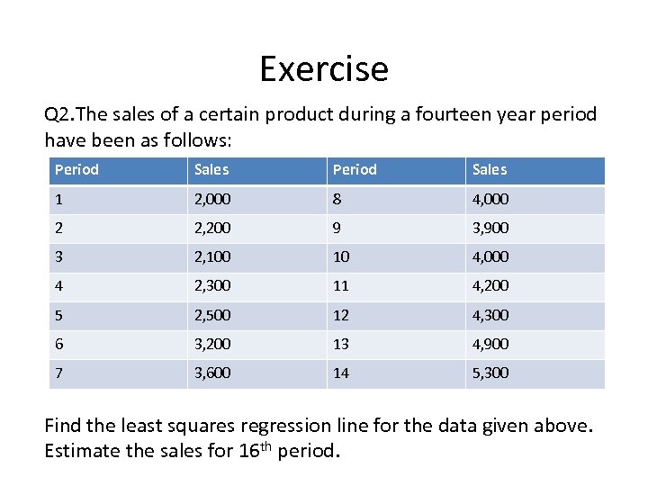
Exercise Q 2. The sales of a certain product during a fourteen year period have been as follows: Period Sales 1 2, 000 8 4, 000 2 2, 200 9 3, 900 3 2, 100 10 4, 000 4 2, 300 11 4, 200 5 2, 500 12 4, 300 6 3, 200 13 4, 900 7 3, 600 14 5, 300 Find the least squares regression line for the data given above. Estimate the sales for 16 th period.

Exercise Q 2. The sales of a certain product during a fourteen year period have been as follows: Period Sales 1 2, 000 8 4, 000 2 2, 200 9 3, 900 3 2, 100 10 4, 000 4 2, 300 11 4, 200 5 2, 500 12 4, 300 6 3, 200 13 4, 900 7 3, 600 14 5, 300 Find the least squares regression line for the data given above. Estimate the sales for 16 th period.
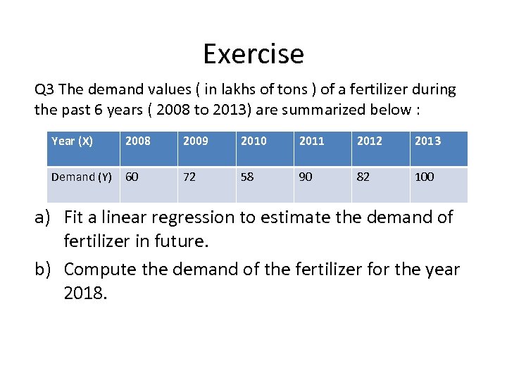
Exercise Q 3 The demand values ( in lakhs of tons ) of a fertilizer during the past 6 years ( 2008 to 2013) are summarized below : Year (X) 2008 2009 2010 2011 2012 2013 Demand (Y) 60 72 58 90 82 100 a) Fit a linear regression to estimate the demand of fertilizer in future. b) Compute the demand of the fertilizer for the year 2018.
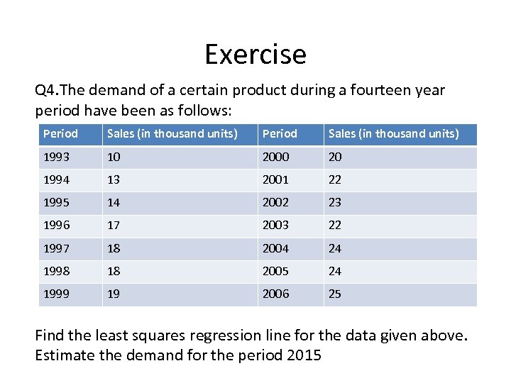
Exercise Q 4. The demand of a certain product during a fourteen year period have been as follows: Period Sales (in thousand units) 1993 10 2000 20 1994 13 2001 22 1995 14 2002 23 1996 17 2003 22 1997 18 2004 24 1998 18 2005 24 1999 19 2006 25 Find the least squares regression line for the data given above. Estimate the demand for the period 2015
00f3b11f3526b145763d4d0497399c5f.ppt