d7722f59271bc6704a2de625c7c40949.ppt
- Количество слайдов: 24
MBA 201 a: Entry, Exit & Equilibrium
Basic definitions & principles (I) • In the short run (SR), – for an individual firm, many costs are sunk, and – for an entire industry, the number of firms is fixed. • In the long run (LR), – everything is variable: production process within a firm and the number of firms. Professor Wolfram MBA 201 a - Fall 2009 Page 1
Basic definitions & principles (II) Profit maximization implies the following decision rules: – In the short run: • Produce at the quantity level where MR=MC*, so long as your revenues cover your variable costs. • Otherwise, exit. – In the long run: • Enter markets or expand capacity as long as your incremental revenues will cover your incremental total costs. • Stay in the market as long as you continue to cover your total costs. • Exit if you can no longer cover your total costs. * Remember that MR=P for a price-taking firm (aka a firm in a perfectly competitive industry). Professor Wolfram MBA 201 a - Fall 2009 Page 2
LR vs. SR example: Recall the t-shirt factory To produce T-shirts: • Lease one machine at $20 / week. • Machine requires one worker. • The machine, operated by the worker, produces one T-shirt per hour. • Worker is paid $1/hour on weekdays (up to 40 hours), $2/hour on Saturdays (up to 8 hours), $3 on Sundays (up to 8 hours). Professor Wolfram MBA 201 a - Fall 2009 Page 3
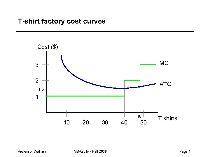
T-shirt factory cost curves Cost ($) MC 3 2 ATC 1. 5 1 48 10 Professor Wolfram 20 30 MBA 201 a - Fall 2009 40 50 T-shirts Page 4
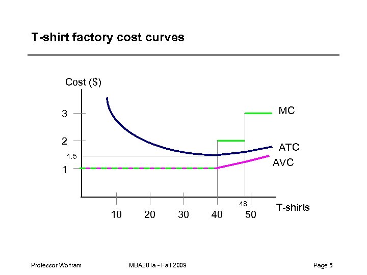
T-shirt factory cost curves Cost ($) MC 3 2 ATC AVC 1. 5 1 48 10 Professor Wolfram 20 30 MBA 201 a - Fall 2009 40 50 T-shirts Page 5
Short versus long run It’s Monday morning. The weekly machine lease has been paid. p=$1. 3. Should the factory shut down? It’s Friday afternoon. Should it pay for next week’s lease? Professor Wolfram MBA 201 a - Fall 2009 Page 6
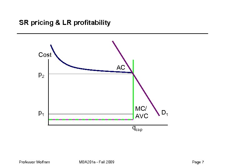
SR pricing & LR profitability Cost AC p 2 MC/ AVC p 1 D 1 qcap Professor Wolfram MBA 201 a - Fall 2009 Page 7
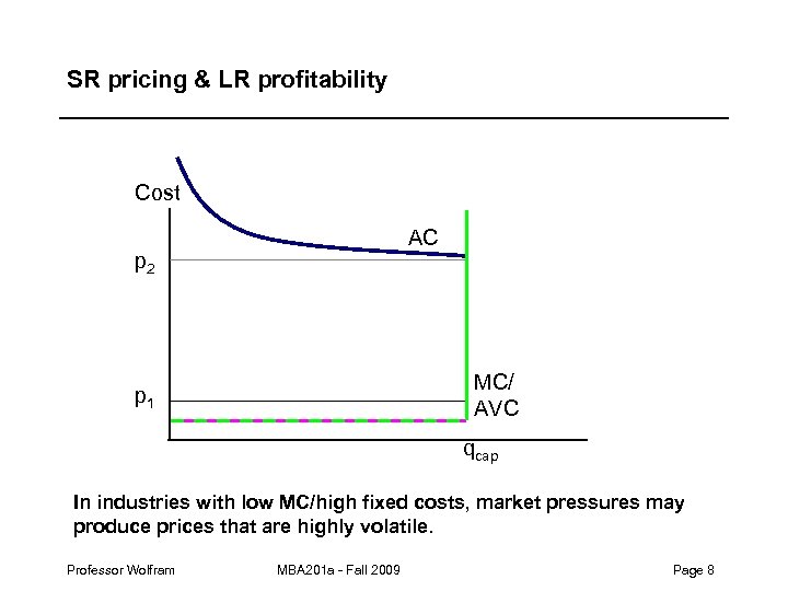
SR pricing & LR profitability Cost AC p 2 MC/ AVC p 1 qcap In industries with low MC/high fixed costs, market pressures may produce prices that are highly volatile. Professor Wolfram MBA 201 a - Fall 2009 Page 8
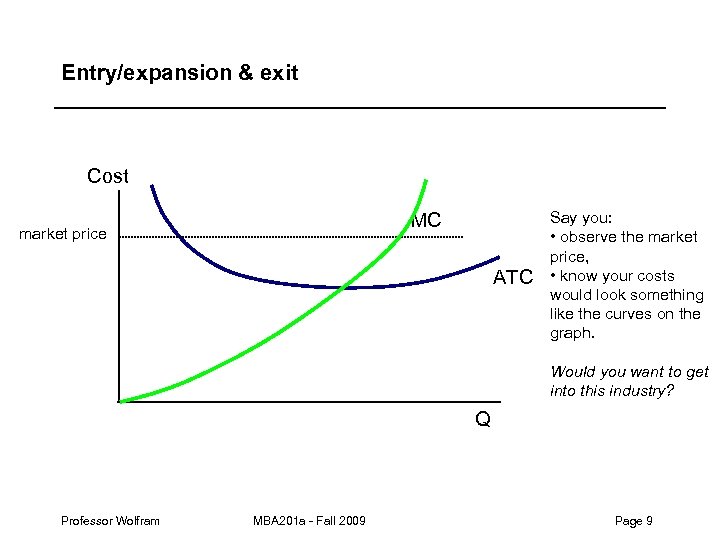
Entry/expansion & exit Cost MC market price ATC Say you: • observe the market price, • know your costs would look something like the curves on the graph. Would you want to get into this industry? Q Professor Wolfram MBA 201 a - Fall 2009 Page 9
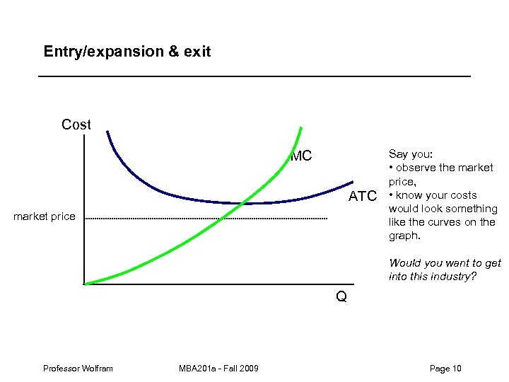
Entry/expansion & exit Cost MC ATC market price Say you: • observe the market price, • know your costs would look something like the curves on the graph. Would you want to get into this industry? Q Professor Wolfram MBA 201 a - Fall 2009 Page 10
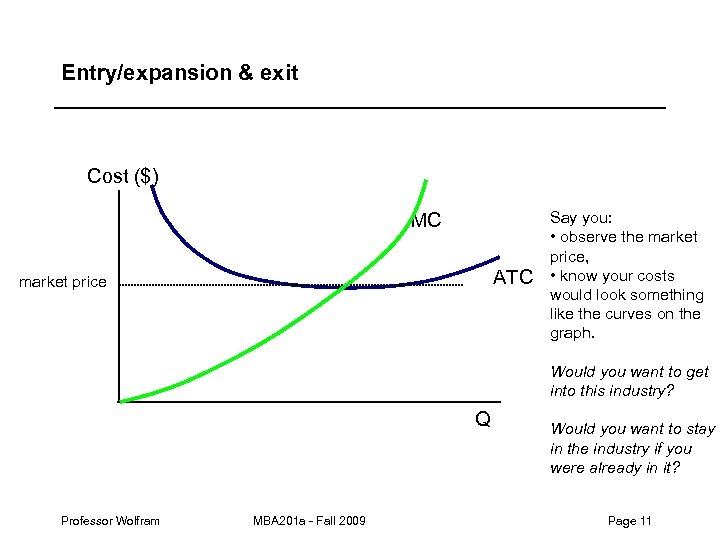
Entry/expansion & exit Cost ($) MC ATC market price Say you: • observe the market price, • know your costs would look something like the curves on the graph. Would you want to get into this industry? Q Professor Wolfram MBA 201 a - Fall 2009 Would you want to stay in the industry if you were already in it? Page 11
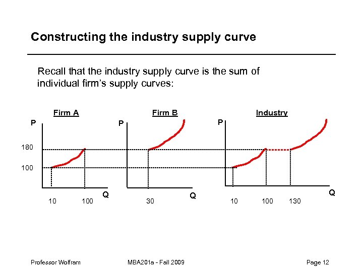
Constructing the industry supply curve Recall that the industry supply curve is the sum of individual firm’s supply curves: Firm A Firm B P Industry P P 180 10 Professor Wolfram 100 Q 30 MBA 201 a - Fall 2009 Q Q 10 100 130 Page 12
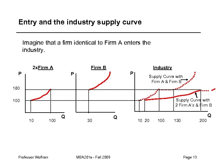
Entry and the industry supply curve Imagine that a firm identical to Firm A enters the industry. 2 x. Firm A Firm B P Industry P P Supply Curve with Firm A & Firm B 180 Supply Curve with 2 Firm A’s & Firm B 100 10 Professor Wolfram 100 Q 30 MBA 201 a - Fall 2009 Q Q 10 20 100 130 200 Page 13
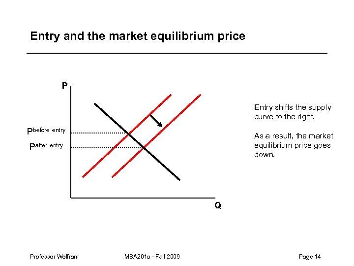
Entry and the market equilibrium price P Entry shifts the supply curve to the right. Pbefore entry As a result, the market equilibrium price goes down. Pafter entry Q Professor Wolfram MBA 201 a - Fall 2009 Page 14
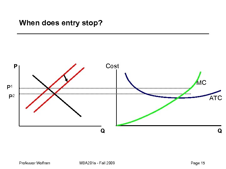
When does entry stop? Cost P MC P 1 P 2 ATC Q Professor Wolfram MBA 201 a - Fall 2009 Q Page 15
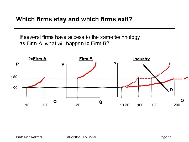
Which firms stay and which firms exit? If several firms have access to the same technology as Firm A, what will happen to Firm B? 2 x. Firm A Firm B P Industry P P 180 100 D 10 Professor Wolfram 100 Q 30 MBA 201 a - Fall 2009 Q Q 10 20 100 130 200 Page 16
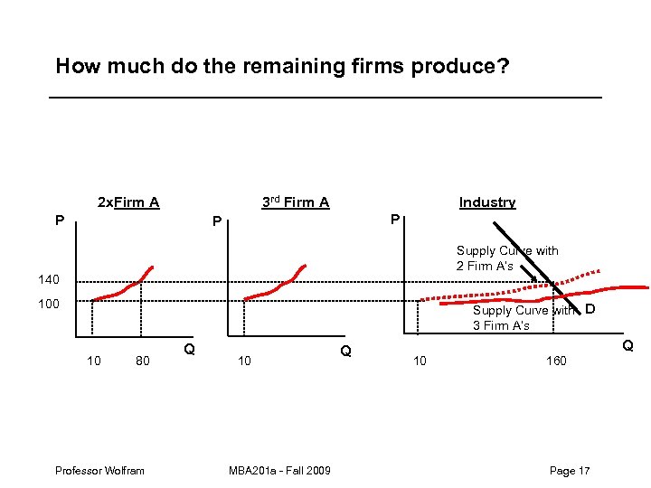
How much do the remaining firms produce? 2 x. Firm A 3 rd Firm A P Industry P P Supply Curve with 2 Firm A’s 140 100 Supply Curve with D 3 Firm A’s 10 80 Professor Wolfram Q 10 MBA 201 a - Fall 2009 Q Q 10 160 Page 17
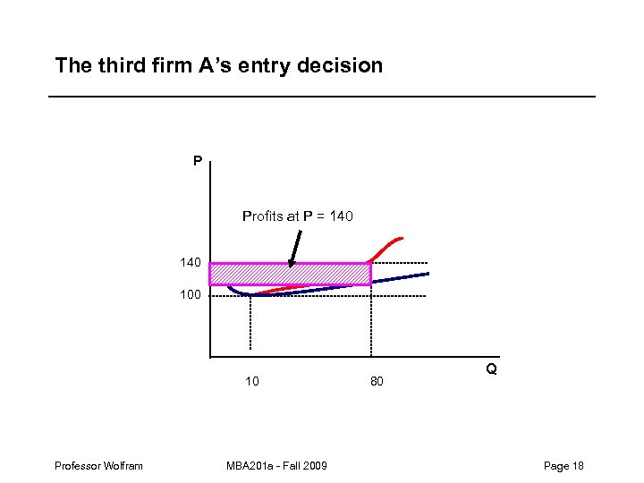
The third firm A’s entry decision P Profits at P = 140 100 10 Professor Wolfram MBA 201 a - Fall 2009 80 Q Page 18
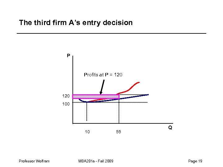
The third firm A’s entry decision P Profits at P = 120 100 10 Professor Wolfram MBA 201 a - Fall 2009 55 Q Page 19
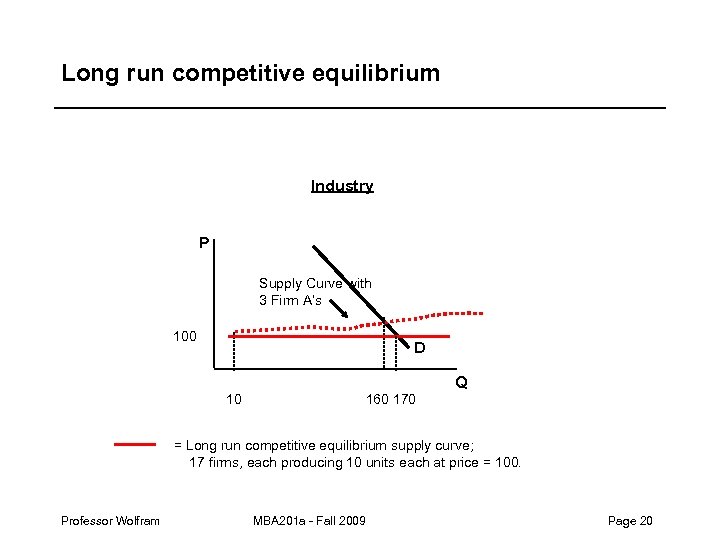
Long run competitive equilibrium Industry P Supply Curve with 3 Firm A’s 100 D Q 10 160 170 = Long run competitive equilibrium supply curve; 17 firms, each producing 10 units each at price = 100. Professor Wolfram MBA 201 a - Fall 2009 Page 20
Long run competitive equilibrium In a long-run competitive equilibrium: – All of the existing firms are maximizing their short-run profits. – None of the existing firms want to either exit or expand output. – No new firms want to enter. – All existing firms earn zero economic profits. – The market price equals the minimum of the long-run average cost curve (P=min(LRAC)). – All consumers who want to buy the product at this price are able to. Professor Wolfram MBA 201 a - Fall 2009 Page 21
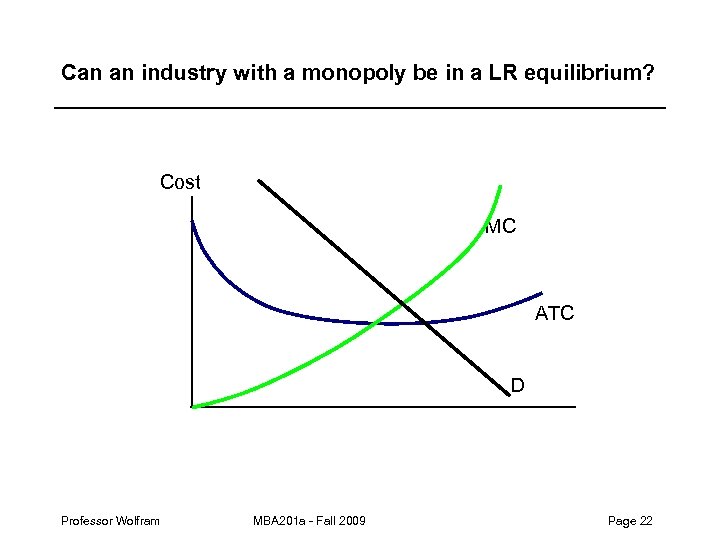
Can an industry with a monopoly be in a LR equilibrium? Cost MC ATC D Professor Wolfram MBA 201 a - Fall 2009 Page 22
Takeaways – Firms have more control over their costs in the long run. – A firm should stay in business in the short run as long as it is making some contribution towards its fixed costs (i. e. P>AVC). – The following dynamics contribute to the long-run competitive equilibrium: • Firms entering markets where there are opportunities to make profits. • Firms exiting markets where they can no longer cover their total costs, even if they’re making profit maximizing price/output decisions. – In a long-run competitive equilibrium: p=min(LRAC), all firms earn zero economic profits. Professor Wolfram MBA 201 a - Fall 2009 Page 23
d7722f59271bc6704a2de625c7c40949.ppt