MATH 2016 13177 Statistical Modelling Course coordinator Chris

MATH 2016 (13177) Statistical Modelling Course coordinator: Chris Brien Course is about designing experiments and using linear models to analyze data, both from experiments and surveys. Statistical Modelling Chapter I 1

I. Statistical inference I. A Expected values and variances I. B The linear regression model I. C Model selection a) Obtaining parameter estimates b) Regression analysis of variance I. D Summary Statistical Modelling Chapter I 4

I. A Expected values and variances • Statistical inference is about drawing conclusions about one or more populations based on samples from the populations. • Compute statistics or estimates from samples. • They are used as estimates of particular population quantities, these being called parameters. • Important to be clear about distinction —when one is talking about a mean, is it the population or sample mean? • To aid in making the distinction, convention is to use Greek letters as symbols for parameters and ordinary Roman letters as symbols for statistics. • Fundamental in this course are population expected value and variance. Statistical Modelling Chapter I 5

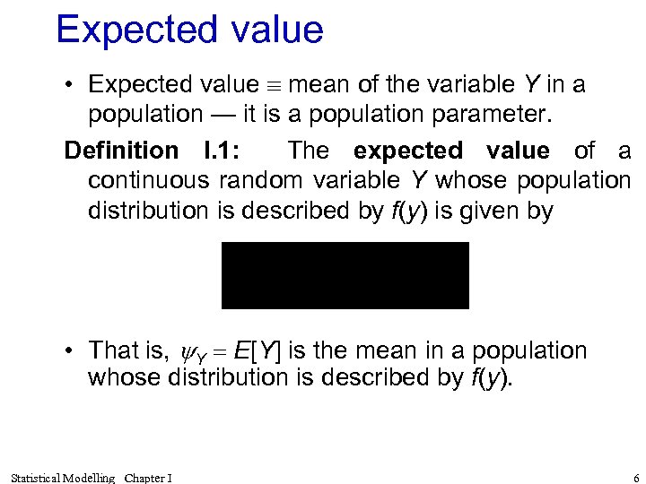Expected value • Expected value mean of the variable Y in a population — it is a population parameter. Definition I. 1: The expected value of a continuous random variable Y whose population distribution is described by f(y) is given by • That is, y. Y = E[Y] is the mean in a population whose distribution is described by f(y). Statistical Modelling Chapter I 6

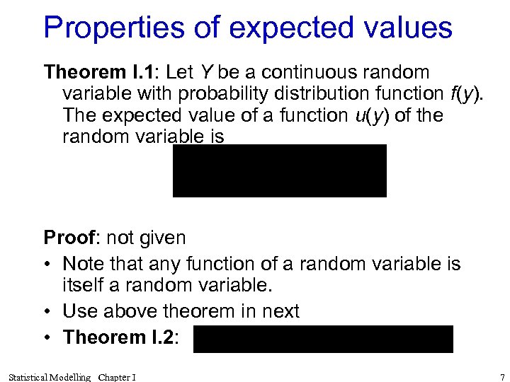Properties of expected values Theorem I. 1: Let Y be a continuous random variable with probability distribution function f(y). The expected value of a function u(y) of the random variable is Proof: not given • Note that any function of a random variable is itself a random variable. • Use above theorem in next • Theorem I. 2: Statistical Modelling Chapter I 7

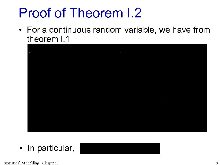Proof of Theorem I. 2 • For a continuous random variable, we have from theorem I. 1 • In particular, Statistical Modelling Chapter I 8

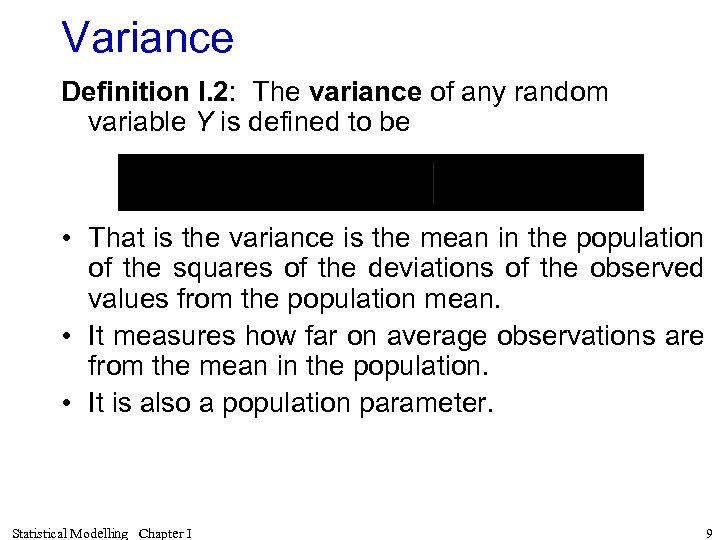Variance Definition I. 2: The variance of any random variable Y is defined to be • That is the variance is the mean in the population of the squares of the deviations of the observed values from the population mean. • It measures how far on average observations are from the mean in the population. • It is also a population parameter. Statistical Modelling Chapter I 9

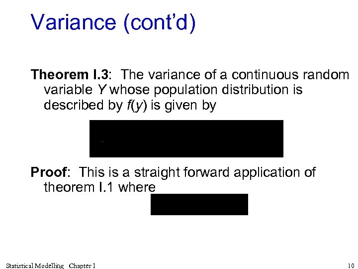Variance (cont’d) Theorem I. 3: The variance of a continuous random variable Y whose population distribution is described by f(y) is given by Proof: This is a straight forward application of theorem I. 1 where Statistical Modelling Chapter I 10

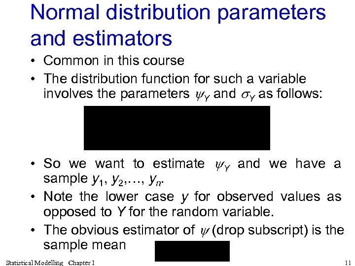Normal distribution parameters and estimators • Common in this course • The distribution function for such a variable involves the parameters y. Y and s. Y as follows: • So we want to estimate y. Y and we have a sample y 1, y 2, …, yn. • Note the lower case y for observed values as opposed to Y for the random variable. • The obvious estimator of y (drop subscript) is the sample mean Statistical Modelling Chapter I 11

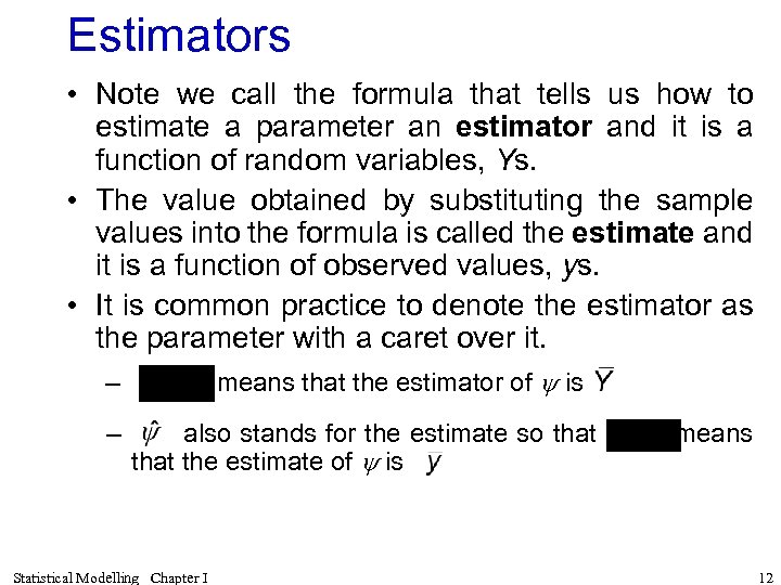Estimators • Note we call the formula that tells us how to estimate a parameter an estimator and it is a function of random variables, Ys. • The value obtained by substituting the sample values into the formula is called the estimate and it is a function of observed values, ys. • It is common practice to denote the estimator as the parameter with a caret over it. – means that the estimator of y is – also stands for the estimate so that means that the estimate of y is Statistical Modelling Chapter I 12

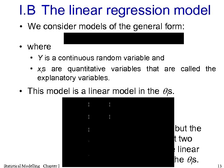I. B The linear regression model • We consider models of the general form: • where • Y is a continuous random variable and • xis are quantitative variables that are called the explanatory variables. • This model is a linear model in the qis. Statistical Modelling Chapter I All but the last two are linear in the qis. 13

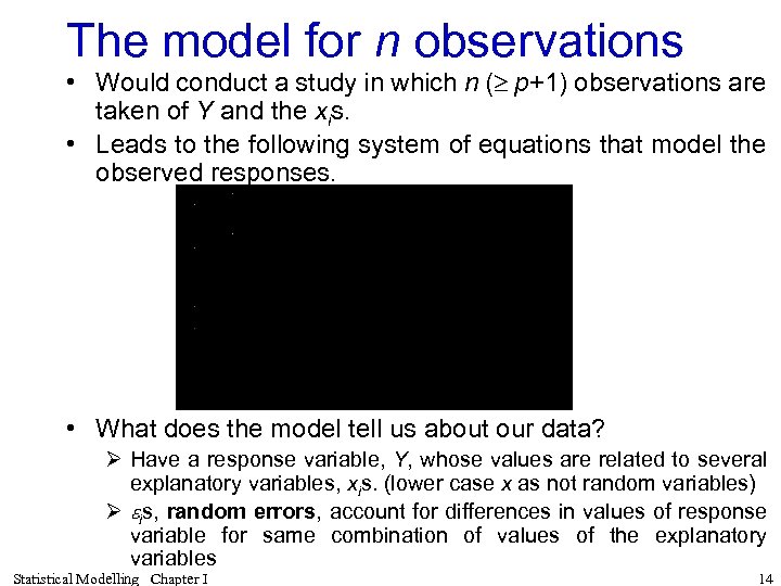The model for n observations • Would conduct a study in which n ( p+1) observations are taken of Y and the xis. • Leads to the following system of equations that model the observed responses. • What does the model tell us about our data? Ø Have a response variable, Y, whose values are related to several explanatory variables, xis. (lower case x as not random variables) Ø eis, random errors, account for differences in values of response variable for same combination of values of the explanatory variables Statistical Modelling Chapter I 14

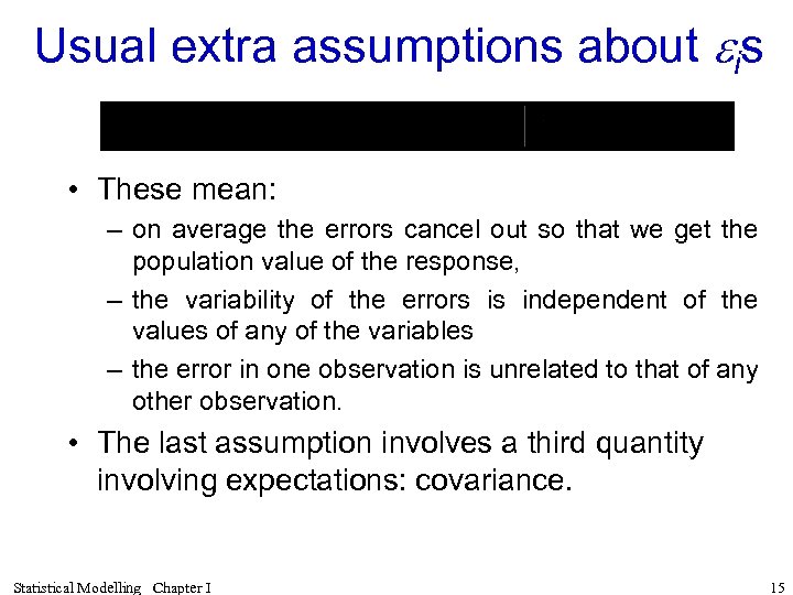Usual extra assumptions about eis • These mean: – on average the errors cancel out so that we get the population value of the response, – the variability of the errors is independent of the values of any of the variables – the error in one observation is unrelated to that of any other observation. • The last assumption involves a third quantity involving expectations: covariance. Statistical Modelling Chapter I 15

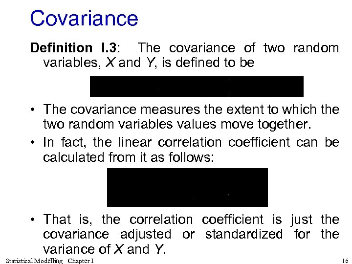Covariance Definition I. 3: The covariance of two random variables, X and Y, is defined to be • The covariance measures the extent to which the two random variables values move together. • In fact, the linear correlation coefficient can be calculated from it as follows: • That is, the correlation coefficient is just the covariance adjusted or standardized for the variance of X and Y. Statistical Modelling Chapter I 16

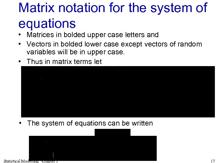Matrix notation for the system of equations • Matrices in bolded upper case letters and • Vectors in bolded lower case except vectors of random variables will be in upper case. • Thus in matrix terms let • The system of equations can be written Statistical Modelling Chapter I 17

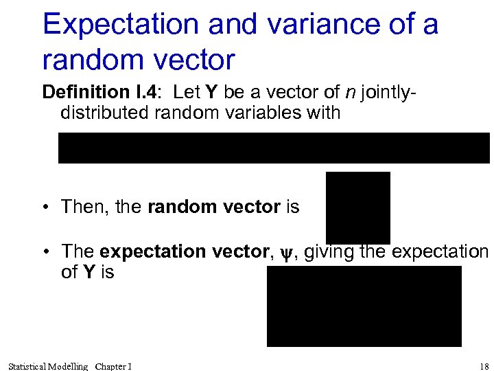Expectation and variance of a random vector Definition I. 4: Let Y be a vector of n jointlydistributed random variables with • Then, the random vector is • The expectation vector, y, giving the expectation of Y is Statistical Modelling Chapter I 18

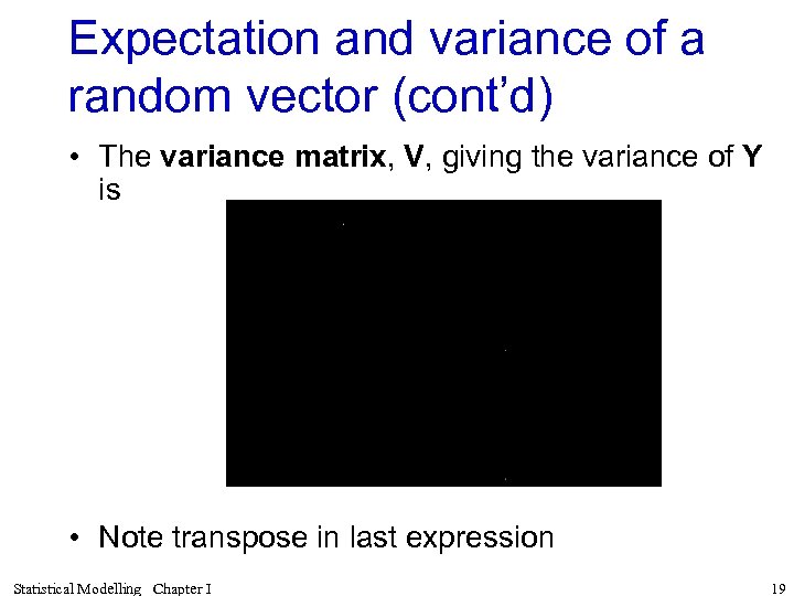Expectation and variance of a random vector (cont’d) • The variance matrix, V, giving the variance of Y is • Note transpose in last expression Statistical Modelling Chapter I 19

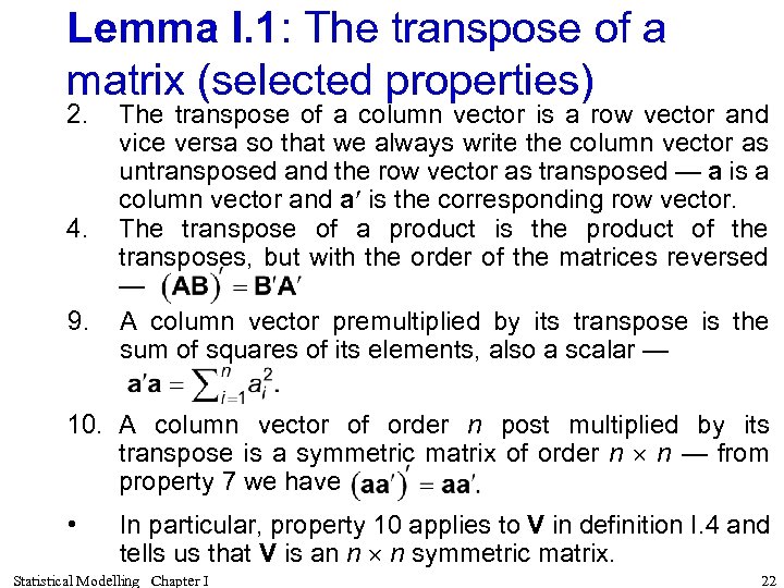Lemma I. 1: The transpose of a matrix (selected properties) 2. 4. 9. The transpose of a column vector is a row vector and vice versa so that we always write the column vector as untransposed and the row vector as transposed — a is a column vector and a is the corresponding row vector. The transpose of a product is the product of the transposes, but with the order of the matrices reversed — A column vector premultiplied by its transpose is the sum of squares of its elements, also a scalar — 10. A column vector of order n post multiplied by its transpose is a symmetric matrix of order n n — from property 7 we have • In particular, property 10 applies to V in definition I. 4 and tells us that V is an n n symmetric matrix. Statistical Modelling Chapter I 22

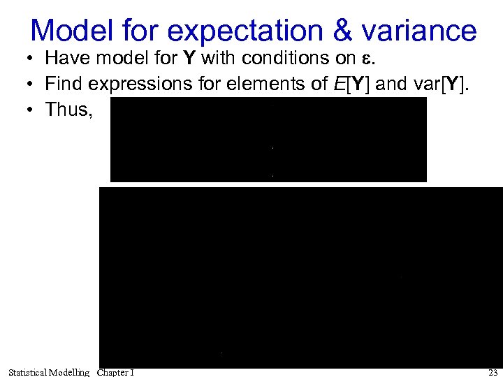Model for expectation & variance • Have model for Y with conditions on e. • Find expressions for elements of E[Y] and var[Y]. • Thus, Statistical Modelling Chapter I 23

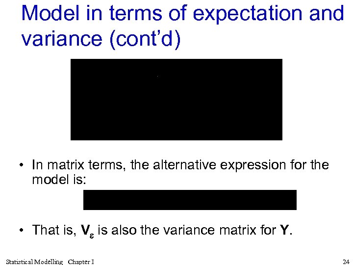Model in terms of expectation and variance (cont’d) • In matrix terms, the alternative expression for the model is: • That is, Ve is also the variance matrix for Y. Statistical Modelling Chapter I 24

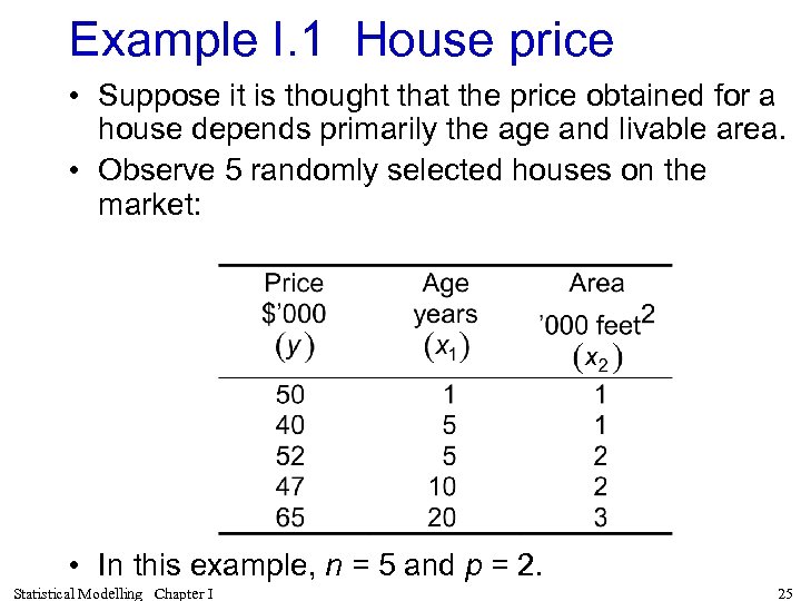Example I. 1 House price • Suppose it is thought that the price obtained for a house depends primarily the age and livable area. • Observe 5 randomly selected houses on the market: • In this example, n = 5 and p = 2. Statistical Modelling Chapter I 25

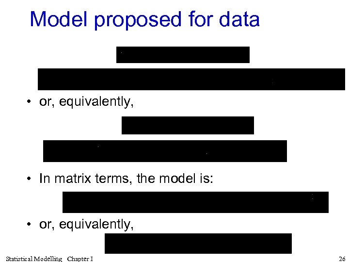Model proposed for data • or, equivalently, • In matrix terms, the model is: • or, equivalently, Statistical Modelling Chapter I 26

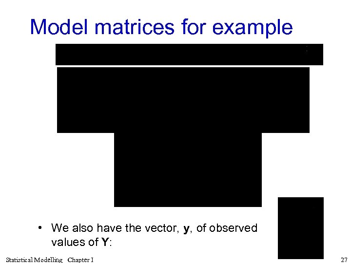Model matrices for example • We also have the vector, y, of observed values of Y: Statistical Modelling Chapter I 27

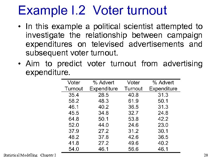Example I. 2 Voter turnout • In this example a political scientist attempted to investigate the relationship between campaign expenditures on televised advertisements and subsequent voter turnout. • Aim to predict voter turnout from advertising expenditure. Statistical Modelling Chapter I 28

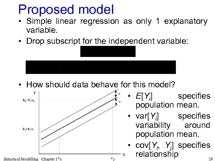Proposed model • Simple linear regression as only 1 explanatory variable. • Drop subscript for the independent variable: • How should data behave for this model? • E[Yi] specifies population mean. • var[Yi] specifies variability around population mean. • cov[Yi, Yj] specifies relationship 29 Statistical Modelling Chapter I

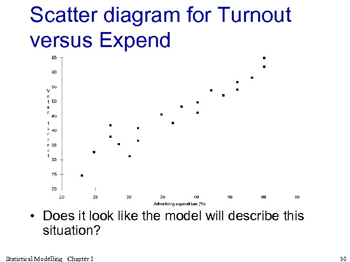Scatter diagram for Turnout versus Expend • Does it look like the model will describe this situation? Statistical Modelling Chapter I 30

I. C Model selection • Generally, we want to determine the model that best describes the data. • To do this we usually obtain estimates of our parameters under several alternative models and use these in deciding which model to use to describe the data. • The choice of models is often made using an analysis of variance (ANOVA). Statistical Modelling Chapter I 31

a) Obtaining parameter estimates • Estimators of the parameters q in the expectation model are obtained using the least squares or maximum likelihood criteria — they are equivalent in the context of linear models. • Also, an estimator of s 2 is obtained from the ANOVA described in the next section. • Here will establish the least squares estimators of q. Statistical Modelling Chapter I 32

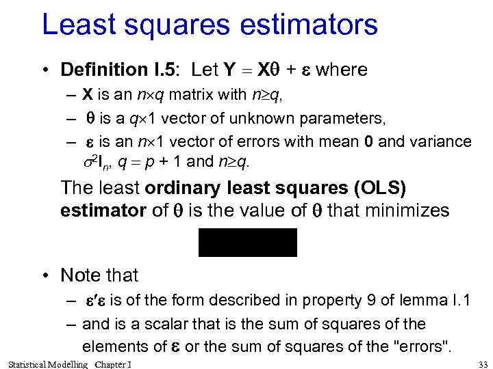Least squares estimators • Definition I. 5: Let Y = Xq + e where – X is an n q matrix with n q, – q is a q 1 vector of unknown parameters, – e is an n 1 vector of errors with mean 0 and variance s 2 In, q = p + 1 and n q. The least ordinary least squares (OLS) estimator of q is the value of q that minimizes • Note that – e e is of the form described in property 9 of lemma I. 1 – and is a scalar that is the sum of squares of the elements of e or the sum of squares of the "errors". Statistical Modelling Chapter I 33

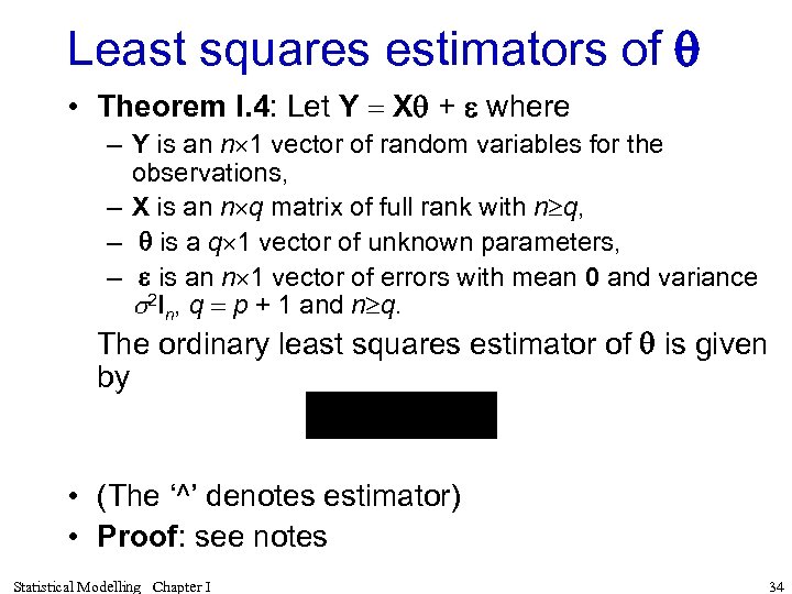Least squares estimators of q • Theorem I. 4: Let Y = Xq + e where – Y is an n 1 vector of random variables for the observations, – X is an n q matrix of full rank with n q, – q is a q 1 vector of unknown parameters, – e is an n 1 vector of errors with mean 0 and variance s 2 In, q = p + 1 and n q. The ordinary least squares estimator of q is given by • (The ‘^’ denotes estimator) • Proof: see notes Statistical Modelling Chapter I 34

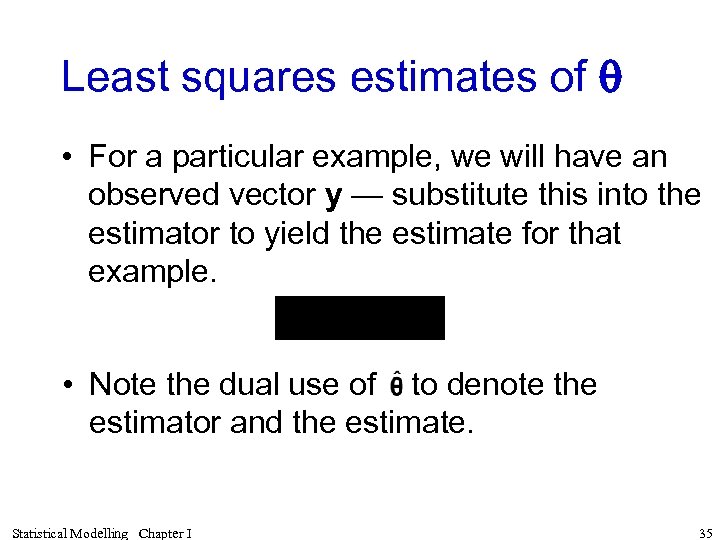Least squares estimates of q • For a particular example, we will have an observed vector y — substitute this into the estimator to yield the estimate for that example. • Note the dual use of to denote the estimator and the estimate. Statistical Modelling Chapter I 35

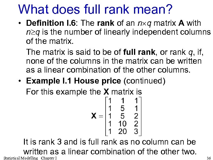What does full rank mean? • Definition I. 6: The rank of an n q matrix A with n q is the number of linearly independent columns of the matrix. The matrix is said to be of full rank, or rank q, if, none of the columns in the matrix can be written as a linear combination of the other columns. • Example I. 1 House price (continued) For this example the X matrix is It is rank 3 and is full rank as no column can be written as a linear combination of the other two. Statistical Modelling Chapter I 36

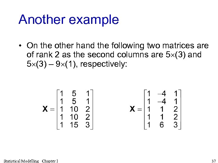Another example • On the other hand the following two matrices are of rank 2 as the second columns are 5 (3) and 5 (3) – 9 (1), respectively: Statistical Modelling Chapter I 37

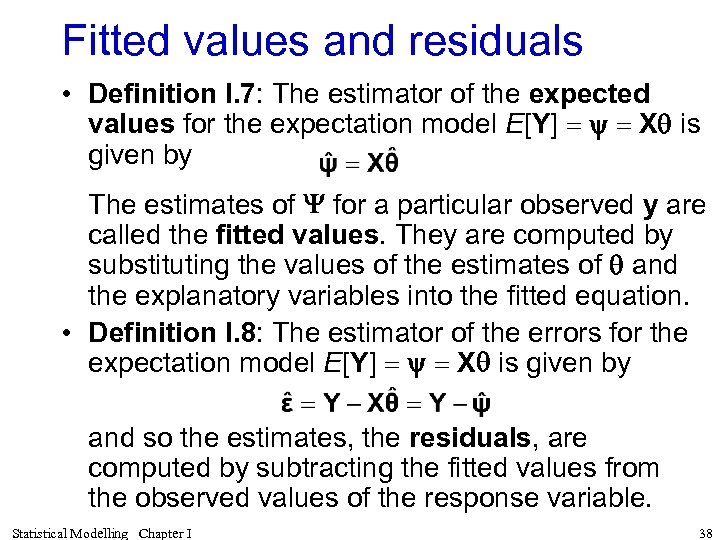Fitted values and residuals • Definition I. 7: The estimator of the expected values for the expectation model E[Y] = y = Xq is given by The estimates of Y for a particular observed y are called the fitted values. They are computed by substituting the values of the estimates of q and the explanatory variables into the fitted equation. • Definition I. 8: The estimator of the errors for the expectation model E[Y] = y = Xq is given by and so the estimates, the residuals, are computed by subtracting the fitted values from the observed values of the response variable. Statistical Modelling Chapter I 38

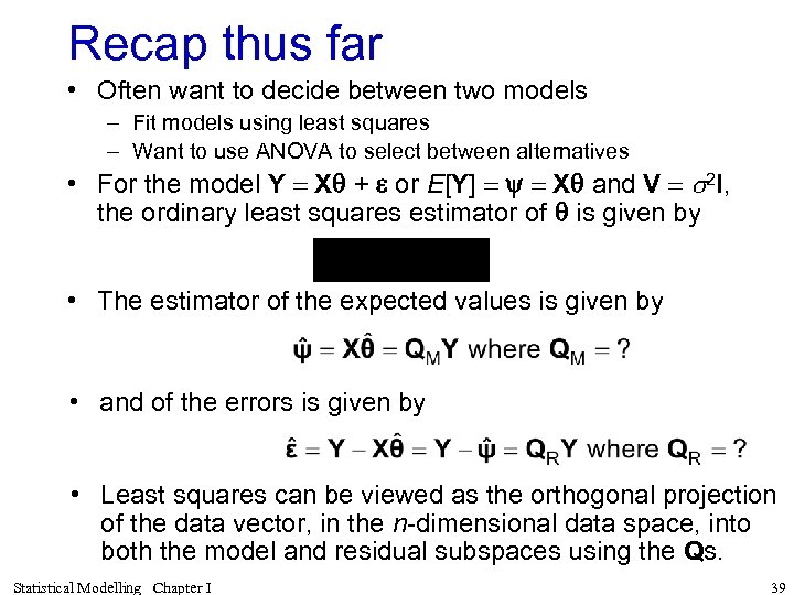Recap thus far • Often want to decide between two models – Fit models using least squares – Want to use ANOVA to select between alternatives • For the model Y = Xq + e or E[Y] = y = Xq and V = s 2 I, the ordinary least squares estimator of q is given by • The estimator of the expected values is given by • and of the errors is given by • Least squares can be viewed as the orthogonal projection of the data vector, in the n-dimensional data space, into both the model and residual subspaces using the Qs. Statistical Modelling Chapter I 39

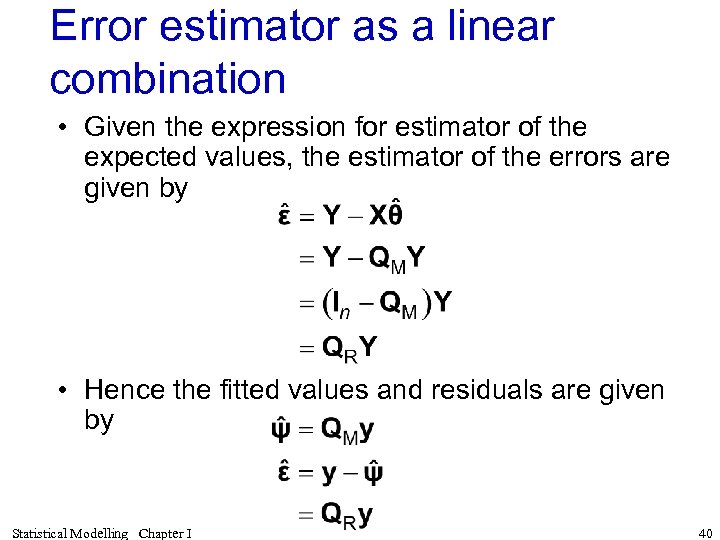Error estimator as a linear combination • Given the expression for estimator of the expected values, the estimator of the errors are given by • Hence the fitted values and residuals are given by Statistical Modelling Chapter I 40

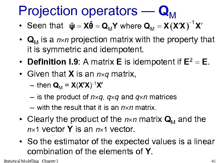Projection operators — QM • Seen that • QM is a n n projection matrix with the property that it is symmetric and idempotent. • Definition I. 9: A matrix E is idempotent if E 2 = E. • Given that X is an n q matrix, – then QM = X(X X)-1 X – is the product of n q, q q and q n matrices – with the result that it is an n n matrix. • Clearly the product of the n n matrix QM and the n 1 vector Y is an n 1 vector. • So the estimator of the expected values is a linear combination of the elements of Y. Statistical Modelling Chapter I 41

Projection operators — QR • Theorem I. 5: Given that the matrix E is symmetric and idempotent, then R = I - E is also symmetric and idempotent. In addition, RE = ER = 0. • Application of this theorem to the regression situation leads us to conclude that – QR is symmetric and idempotent – with QRQM = QMQR = 0. • All of this can be viewed as the orthogonal projection of vectors onto subspaces. Statistical Modelling Chapter I 42

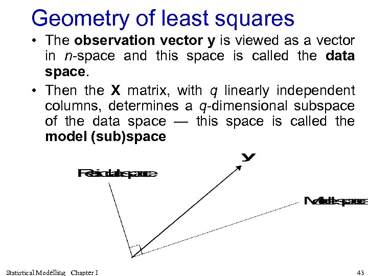Geometry of least squares • The observation vector y is viewed as a vector in n-space and this space is called the data space. • Then the X matrix, with q linearly independent columns, determines a q-dimensional subspace of the data space — this space is called the model (sub)space Statistical Modelling Chapter I 43

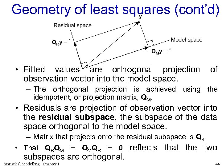Geometry of least squares (cont’d) • Fitted values are orthogonal projection of observation vector into the model space. – The orthogonal projection is achieved using the idempotent, or projection matrix, QM. • Residuals are projection of observation vector into the residual subspace, the subspace of the data space orthogonal to the model space. – Matrix that projects onto the residual subspace is QR. • That QRQM = QMQR = 0 reflects that the two subspaces are orthogonal. Statistical Modelling Chapter I 44

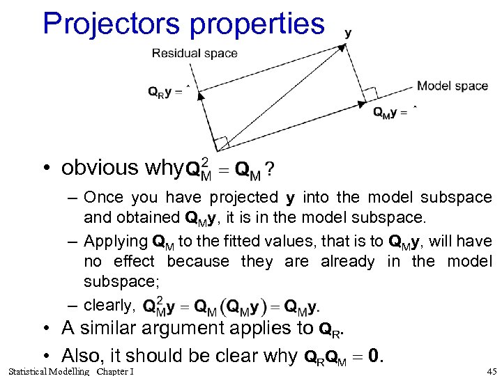Projectors properties • obvious why – Once you have projected y into the model subspace and obtained QMy, it is in the model subspace. – Applying QM to the fitted values, that is to QMy, will have no effect because they are already in the model subspace; – clearly, • A similar argument applies to QR. • Also, it should be clear why QRQM = 0. Statistical Modelling Chapter I 45

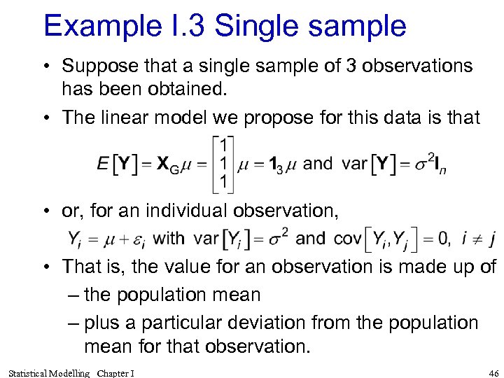Example I. 3 Single sample • Suppose that a single sample of 3 observations has been obtained. • The linear model we propose for this data is that • or, for an individual observation, • That is, the value for an observation is made up of – the population mean – plus a particular deviation from the population mean for that observation. Statistical Modelling Chapter I 46

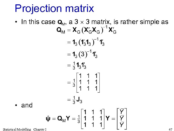Projection matrix • In this case QM, a 3 3 matrix, is rather simple as • and Statistical Modelling Chapter I 47

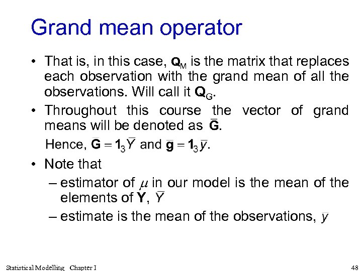Grand mean operator • That is, in this case, QM is the matrix that replaces each observation with the grand mean of all the observations. Will call it QG. • Throughout this course the vector of grand means will be denoted as . • Note that – estimator of m in our model is the mean of the elements of Y, – estimate is the mean of the observations, Statistical Modelling Chapter I 48

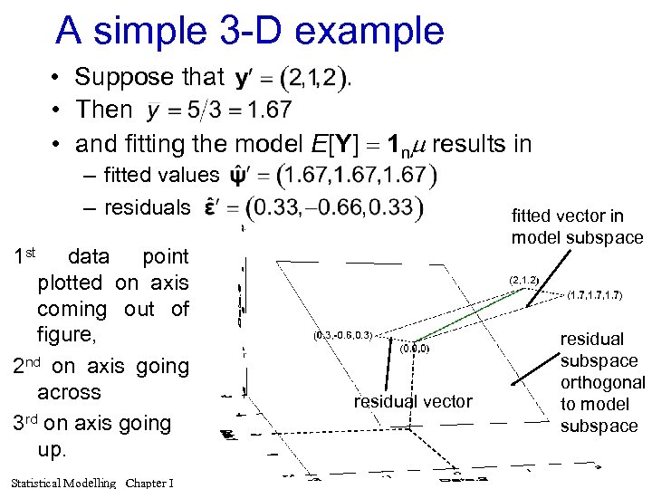A simple 3 -D example • Suppose that • Then • and fitting the model E[Y] = 1 nm results in – fitted values – residuals 1 st data point plotted on axis coming out of figure, 2 nd on axis going across 3 rd on axis going up. Statistical Modelling Chapter I fitted vector in model subspace residual vector residual subspace orthogonal to model subspace 49

I. C Model selection • Generally, we want to determine the model that best describes the data. – obtain estimates of our parameters under several alternative models. – Choose model using an analysis of variance (ANOVA). Statistical Modelling Chapter I 50

b) Regression analysis of variance • An ANOVA is used to compare potential models. • In the case of the regression model, it is common to want to choose between two expectation models, one which is a subset of the other. Statistical Modelling Chapter I 52

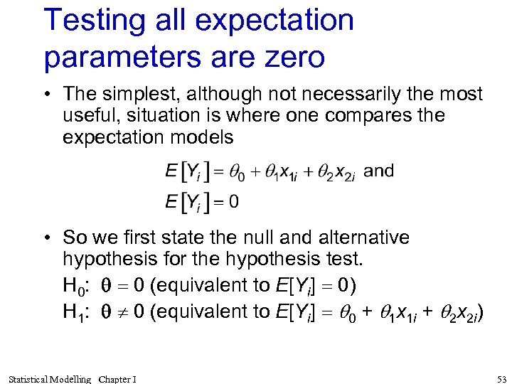Testing all expectation parameters are zero • The simplest, although not necessarily the most useful, situation is where one compares the expectation models • So we first state the null and alternative hypothesis for the hypothesis test. H 0: q = 0 (equivalent to E[Yi] = 0) H 1: q 0 (equivalent to E[Yi] = q 0 + q 1 x 1 i + q 2 x 2 i) Statistical Modelling Chapter I 53

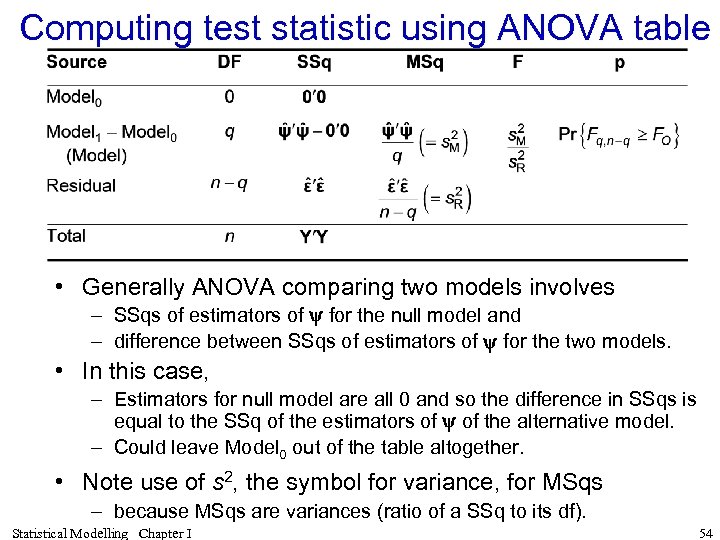Computing test statistic using ANOVA table • Generally ANOVA comparing two models involves – SSqs of estimators of y for the null model and – difference between SSqs of estimators of y for the two models. • In this case, – Estimators for null model are all 0 and so the difference in SSqs is equal to the SSq of the estimators of y of the alternative model. – Could leave Model 0 out of the table altogether. • Note use of s 2, the symbol for variance, for MSqs – because MSqs are variances (ratio of a SSq to its df). Statistical Modelling Chapter I 54

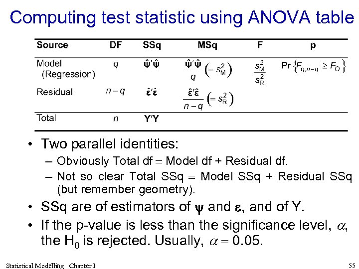Computing test statistic using ANOVA table • Two parallel identities: – Obviously Total df = Model df + Residual df. – Not so clear Total SSq = Model SSq + Residual SSq (but remember geometry). • SSq are of estimators of y and e, and of Y. • If the p-value is less than the significance level, a, the H 0 is rejected. Usually, a = 0. 05. Statistical Modelling Chapter I 55

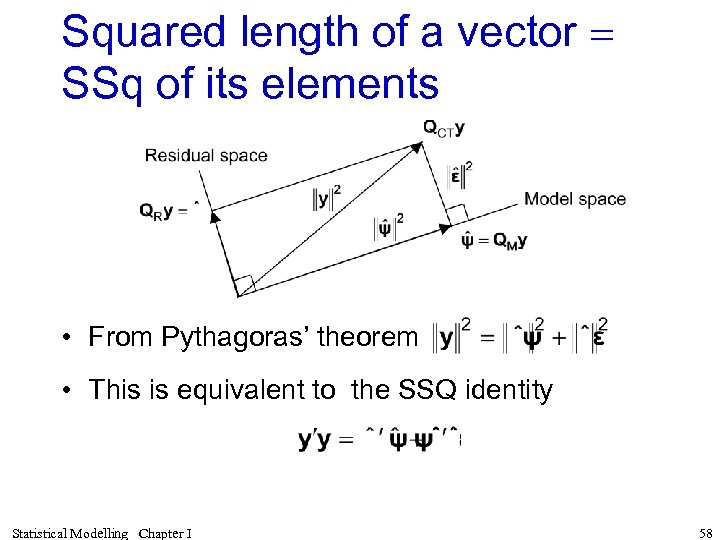Squared length of a vector = SSq of its elements • From Pythagoras’ theorem • This is equivalent to the SSQ identity Statistical Modelling Chapter I 58

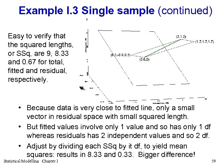Example I. 3 Single sample (continued) Easy to verify that the squared lengths, or SSq, are 9, 8. 33 and 0. 67 for total, fitted and residual, respectively. • Because data is very close to fitted line, only a small vector in residual space with small squared length. • But fitted values involve only 1 value and so has only 1 df whereas residuals has 2 independent values and so 2 df. • Adjust by dividing each SSq by it df, to yield mean squares: results in 8. 33 and 0. 33. Bigger difference! Statistical Modelling Chapter I 59

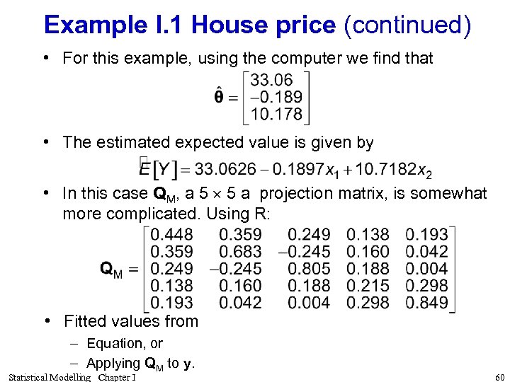Example I. 1 House price (continued) • For this example, using the computer we find that • The estimated expected value is given by • In this case QM, a 5 5 a projection matrix, is somewhat more complicated. Using R: • Fitted values from – Equation, or – Applying QM to y. Statistical Modelling Chapter I 60

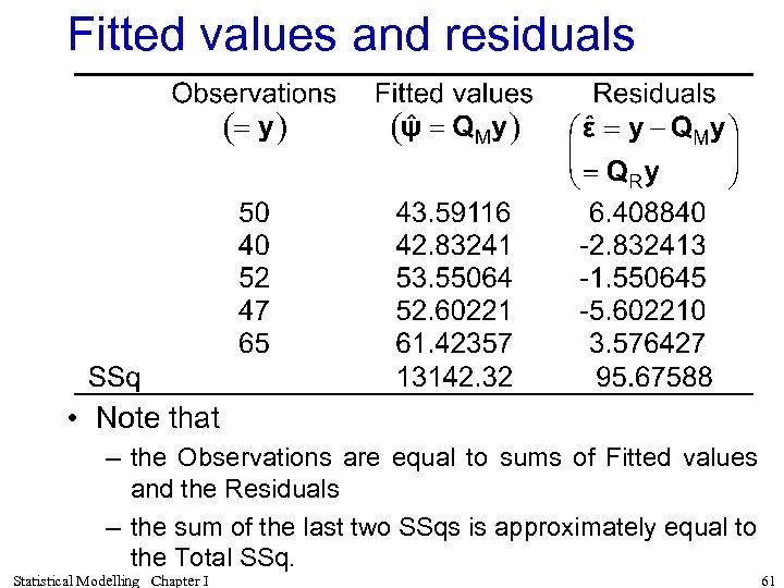Fitted values and residuals • Note that – the Observations are equal to sums of Fitted values and the Residuals – the sum of the last two SSqs is approximately equal to the Total SSq. Statistical Modelling Chapter I 61

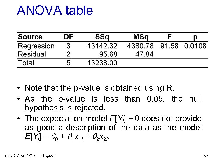ANOVA table • Note that the p-value is obtained using R. • As the p-value is less than 0. 05, the null hypothesis is rejected. • The expectation model E[Yi] = 0 does not provide as good a description of the data as the model E[Yi] = q 0 + q 1 x 1 i + q 2 x 2 i. Statistical Modelling Chapter I 62

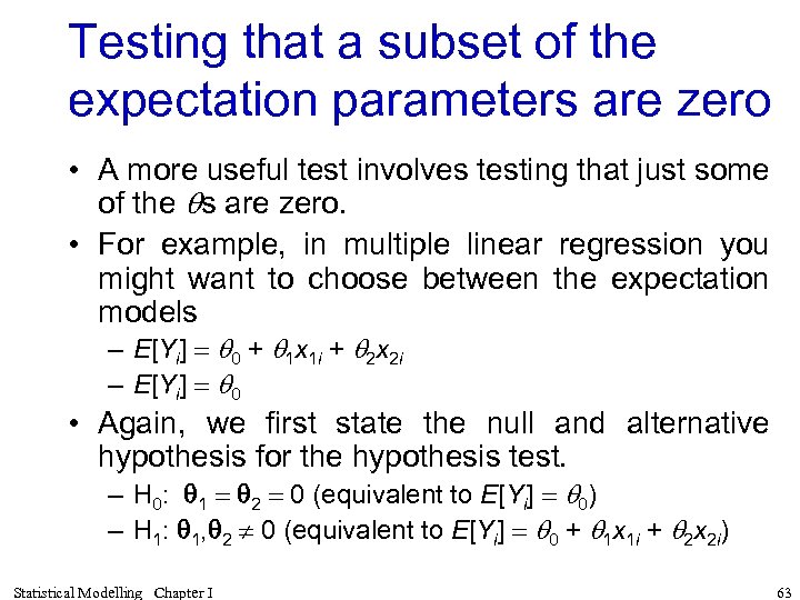Testing that a subset of the expectation parameters are zero • A more useful test involves testing that just some of the qs are zero. • For example, in multiple linear regression you might want to choose between the expectation models – E[Yi] = q 0 + q 1 x 1 i + q 2 x 2 i – E[Yi] = q 0 • Again, we first state the null and alternative hypothesis for the hypothesis test. – H 0: q 1 = q 2 = 0 (equivalent to E[Yi] = q 0) – H 1: q 1, q 2 0 (equivalent to E[Yi] = q 0 + q 1 x 1 i + q 2 x 2 i) Statistical Modelling Chapter I 63

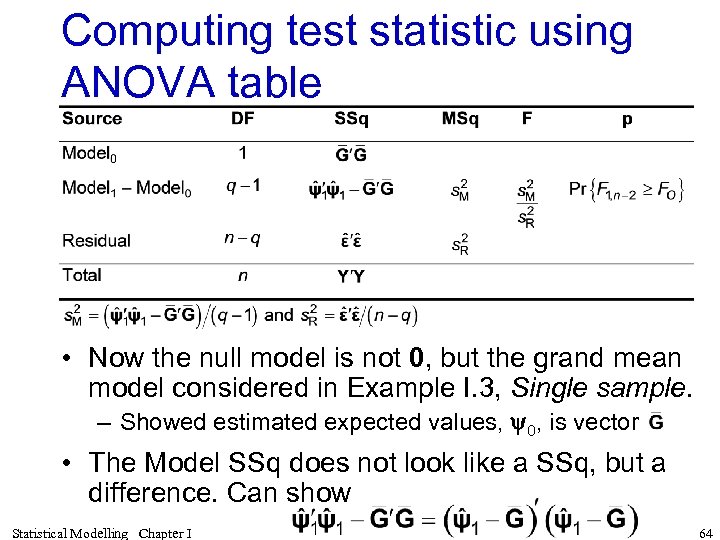Computing test statistic using ANOVA table • Now the null model is not 0, but the grand mean model considered in Example I. 3, Single sample. – Showed estimated expected values, y 0, is vector • The Model SSq does not look like a SSq, but a difference. Can show Statistical Modelling Chapter I 64

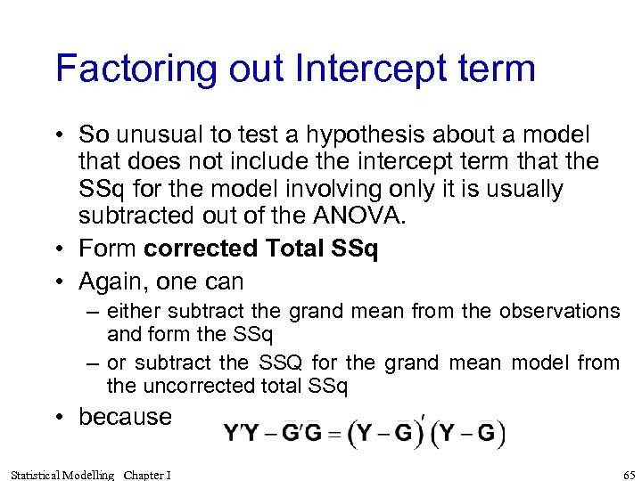Factoring out Intercept term • So unusual to test a hypothesis about a model that does not include the intercept term that the SSq for the model involving only it is usually subtracted out of the ANOVA. • Form corrected Total SSq • Again, one can – either subtract the grand mean from the observations and form the SSq – or subtract the SSQ for the grand mean model from the uncorrected total SSq • because Statistical Modelling Chapter I 65

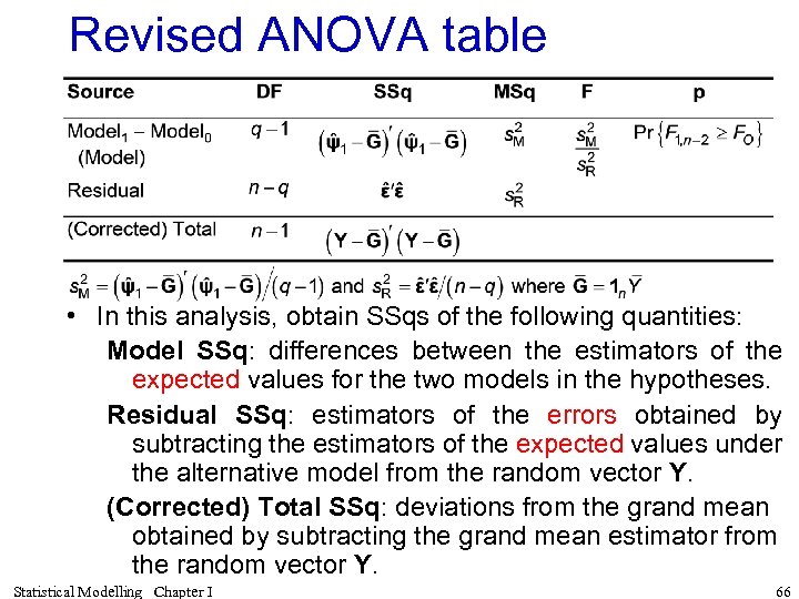Revised ANOVA table • In this analysis, obtain SSqs of the following quantities: Model SSq: differences between the estimators of the expected values for the two models in the hypotheses. Residual SSq: estimators of the errors obtained by subtracting the estimators of the expected values under the alternative model from the random vector Y. (Corrected) Total SSq: deviations from the grand mean obtained by subtracting the grand mean estimator from the random vector Y. Statistical Modelling Chapter I 66

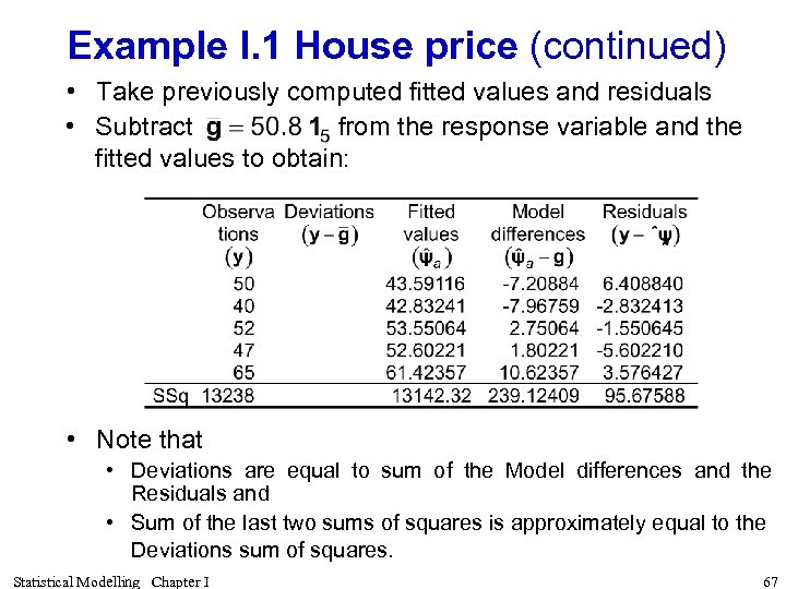Example I. 1 House price (continued) • Take previously computed fitted values and residuals • Subtract from the response variable and the fitted values to obtain: • Note that • Deviations are equal to sum of the Model differences and the Residuals and • Sum of the last two sums of squares is approximately equal to the Deviations sum of squares. Statistical Modelling Chapter I 67

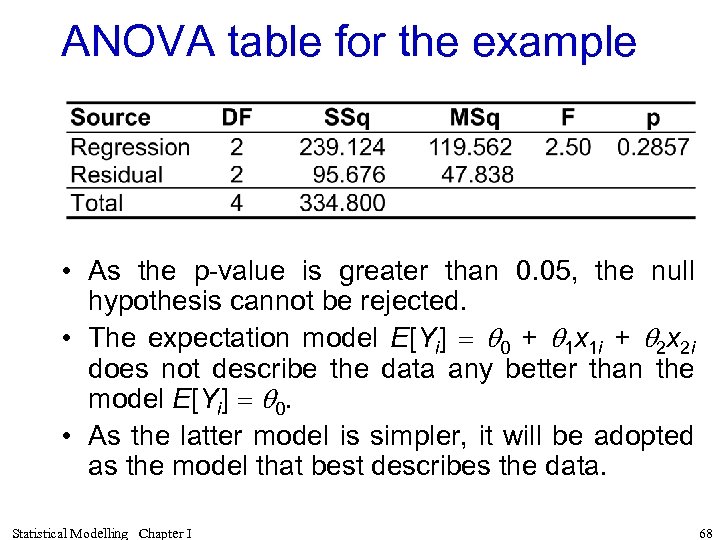ANOVA table for the example • As the p-value is greater than 0. 05, the null hypothesis cannot be rejected. • The expectation model E[Yi] = q 0 + q 1 x 1 i + q 2 x 2 i does not describe the data any better than the model E[Yi] = q 0. • As the latter model is simpler, it will be adopted as the model that best describes the data. Statistical Modelling Chapter I 68

I. E Exercises • There are exercises at the end of the chapter that review the material covered in this chapter. Statistical Modelling Chapter I 69